Introduction
Second sound is a temperature or entropy wave that propagates inside a quantum superfluid, contrasted to the usual density wave of first sound [1]. It is the hallmark of superfluidity: the second sound velocity directly relates to the superfluid fraction, which measures the number of particles undergoing quantum frictionless motion without costing energy, while the second sound attenuation links to the transport coefficients that characterize the momentum and heat transport [1]. Due to the crucial role of second sound played in quantum superfluids, its observation and characterization are one of the most important research goals in the studies of ultracold atomic quantum gases [2].
For a strongly interacting unitary Fermi gas with a divergent s-wave scattering length (a=∞ or 1/a=0) [3], the search for second sound started soon after its realization in 2002 [4]. By using a broad Feshbach resonance located near B≃832 G [5], O’Hara and his colleagues at Duke University successfully demonstrated the ballistic hydrodynamic expansion of a Fermi cloud of lithium atoms, due to either the superfluid hydrodynamics or normal collisional hydrodynamics [4]. This observation paves the way to second sound, if the superfluid hydrodynamics is responsible for the ballistic expansion. Collective density oscillations (i.e., first sounds) of the strongly interacting Fermi gas in harmonic traps were subsequently measured [6–8]. The resulting breathing mode frequency was found to be well explained by the superfluid hydrodynamic theory [9–11]. However, there was no trace of second sound in the measurement of collective density excitations. Theoretical support was not favorable either, since one needs to solve Landau’s two-fluid hydrodynamic equations in the presence of a harmonic trapping potential, which turns out to be fairly non-trivial [12].
This theoretical technical problem was partly solved by Allan Griffin and his co-workers [13–15], by reformulating the dissipationless two-fluid hydrodynamic theory into a variational form [13]. As inspired by the successful confirmation of Fermi superfluidity via the measurements of condensate fraction [16, 17] and vortex lattices [18], more accurate predictions were obtained for the superfluid density [19] and equations of state [20], within the framework of the Gaussian pair fluctuation theory [20]. These predictions provided a useful input to the variational solution of the two-fluid hydrodynamic equations [14]. As a result, various hydrodynamic modes in an isotropic harmonic trap were solved and classified as the first sound and second sound [15]. A major encouraging outcome of this analysis was that, the Landau-Placzek ratio, which characterizes the coupling between first and second sounds was found to be significant for a unitary Fermi gas. Therefore, in principle, one should be able to find the signal of second sound in the density response, by fine tuning the density perturbation close to the avoided crossing of first and second sounds [15].
Experimentally, however, it is difficult to construct a perfectly spherical harmonic trap. For a general axially symmetric harmonic trap, the variational solution of the two-fluid hydrodynamic equations is not available, since too many variational parameters are needed to obtain a convergent solution. To overcome this difficulty, Sandro Stringari and his collaborators proposed to consider a highly elongated cigar trap, for which it is plausible to reduce the three-dimensional two-fluid hydrodynamic equations into an effective one-dimensional form [21, 22]. This brilliant idea turns out to be very successful and eventually leads to the first observation of the second sound propagation in a highly elongated unitary Fermi gas by Sidorenkov and his colleagues at the University of Innsbruck in 2013 [23]. The temperature dependence of superfluid density of the unitary Fermi gas was extracted for the first time. However, the second sound attenuation and the related transport coefficients remain undetermined. This is partly because the reduced one-dimensional hydrodynamic equations are dissipationless [21, 22]. It is not clear how to extract the transport coefficients, even if one can measure the sound attenuation in highly-elongated harmonic traps.
Therefore, harmonic trap potential is very unfriendly to the second sound measurement. Remarkably, recent technical advances enable the realization of a uniform box-trap potential [24]. The experimental manipulation of a homogeneous unitary Fermi gas has now been reported by several groups [25, 26]. In addition to this technical advance, new knowledge of the transport coefficients is also obtained. The shear viscosity of the unitary Fermi gas has been both measured via ballistic expansion [27, 28] and calculated by strong-coupling pair fluctuation theory [29], and the thermal conductivity has been considered [30, 31]. As summarized by two of the present authors in a recent theoretical analysis [32], these developments are promising towards the full characterization of the second sound propagation in uniform traps.
In this year (2022), such a dream came true. This feat was accomplished by Li and his colleagues at the University of Science and Technology of China (USTC) [33], by creating a uniform unitary Fermi gas of lithium atoms with a fairly large Fermi energy and by applying a novel high-resolution Bragg spectroscopy. The superfluid density has been directly measured, with better accuracy. All the transport coefficients are also successfully determined.
It is fairly non-trivial to take nearly twenty years to fully characterize the second sound in a strongly interacting unitary Fermi gas. Interestingly, this is not the end of the journey. The measurements at USTC reveal an impressive sudden rise in the second sound attenuation and thermal conductivity near the superfluid phase transition, which can be viewed as a precursor of critical divergence anticipated near quantum criticality. Future exploration of the quantum critical region with improved temperature controllability may open a new era for studying universal critical dynamics in the strongly interacting regime.
The technique of a uniform box-trap potential also enables the realization of homogeneous interacting Bose-Einstein condensate (BEC) in two and three dimensions. In both cases, the propagation of second sound was observed [34, 35]. The second sound attenuation however may hardly be accurately determined, due to the atom loss at the relatively large s-wave scattering length, which is necessary to bring the system into the hydrodynamic regime.
The rest of the short review is organized as follows. In the next chapter (Section 2), we present Landau’s two-fluid hydrodynamic theory, and briefly discuss the key features of second sound in strongly interacting superfluid helium, particularly near the quantum critical regime. In Section 3, we then introduce the earlier theoretical treatments of the second sound of a unitary Fermi gas in harmonic trap, based on the variational reformulation of the two-fluid hydrodynamic theory. In Sections 4 and 5, we discuss respectively the two milestone experiments on the observation of the second sound propagation and on the measurement of the second sound attenuation in the inhomogeneous and homogeneous unitary Fermi gases, respectively. In Section 6, we summarize the second sound measurements in weakly interacting Bose gases. Finally, Section 7 is devoted to the conclusions and outlooks for some open questions.
Second sound in superfluid helium
We start by discussing the second sound in superfluid helium. The existence of a peculiar second sound was predicted by Laszlo Tisza [36], who first presented the two-fluid hydrodynamic theory of superfluid helium in 1938. Tisza pictured the superfluid helium as having two miscible fluids, the superfluid and normal fluid, which have independent density (ns and nn), and move with different velocities (vs and vn) and without mutual interactions. The superfluid does not carry entropy and flows without dissipation, while the normal fluid carries all the entropy and does have a finite viscosity η. The total density n of superfluid helium is given by the sum of the superfluid density and the normal-fluid density: n=ns+nn.
A direct consequence of the two interpenetrating fluids is that we may have two different sound waves, as illustrated in Fig. 1. First sound is an ordinary sound wave consisting of fluctuations in total density n, in which the superfluid and normal fluid are locked together to undergo an in-phase motion. It depends very weakly on the temperature. In contrast, in another sound wave the superfluid and normal fluid take an out-of-phase motion against each other. As the total density remains constant to first order, the out-of-phase motion leads to fluctuations in relative density and hence in entropy. This creates the entropy wave or temperature wave, which was named as second sound by Lev Landau.
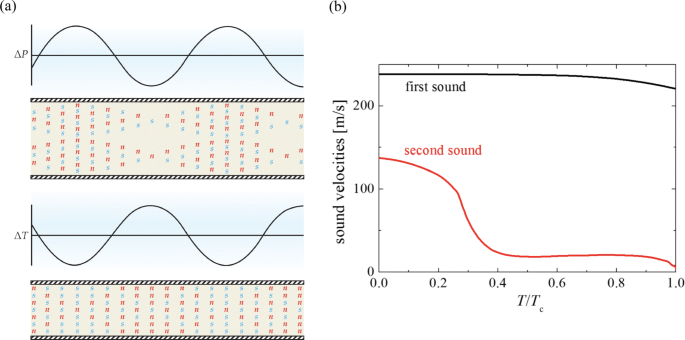
a The characteristics of the two sounds: the in-phase motion (first sound) and the out-of-phase motion (second sound) between the normal and superfluid components, which are shown by the red circles with “n” and the blue circles with “s”. b First and sound velocities of superfluid helium as a function of the reduced temperature T/Tc, where Tc≃2.17 K is the critical temperature. Adapted from Ref. [1] and Ref. [15]
The prediction of second sound is a testbed for the two-fluid hydrodynamic theory. The measurement of second sound velocity turns out to be crucial, in order to correctly understand how the normal-fluid component forms. In 1944, second sound of superfluid helium was successfully detected by Vasilii Peshkov using a standing-wave technique [37]. To fully account for the observed temperature dependence of the second sound velocity for temperatures down to 0.4 K (see the red curve in Fig. 1), we could apply the celebrated two-fluid hydrodynamic equations that were extensively developed by Lev Landau in 1941 [38, 39]:
where j=m(nsvs+nnvn) is the current density, μ is the chemical potential, P is the pressure, and s is the entropy density. The terms on the right-hand side of equations stand for dissipation: η and κ are the shear viscosity and thermal conductivity, respectively, and Γik≡(∂kvni+∂ivnk−2δik∂jvnj/3). For simplicity, we have omitted various second viscosity terms. We have also kept only linear terms in the velocities, which is appropriate for the small-amplitude dynamics such as sound waves. We can then neglect the relative velocity dependence of the thermodynamic quantities and use the standard Gibbs-Duhem relation, i.e., ndμ=−sdT+dP. An external trapping potential Vext is introduced for later convenience. For superfluid helium, it can be understood as the potential from the container wall, and we can set Vext=0 by considering the thermodynamic limit.
Second sound velocity
In this case, we can look for the small-amplitude solutions that vary in space and time like plane-waves (i.e., δn,δT∝ei(k·r−ωt)) and therefore expand all the thermodynamic quantities around their equilibrium values. After some lengthy but straightforward manipulation, we obtain the equation for the sound velocities in the absence of dissipation [39]:
where \(v_{S}=\sqrt {(\partial P/\partial n)_{\bar {s}}/m}\) and \(v_{T}=\sqrt {(\partial P/\partial n)_{T}/m}\) are respectively the adiabatic and isothermal sound velocities, and we have also defined:
with the entropy per particle \(\bar {s}\equiv s/n\) and the specific heat per particle at constant volume \(\bar {c}_{V}=T(\partial \bar {s}/\partial T)_{T}\). By using the thermodynamic relation, \(v_{S}^{2}/v_{T}^{2}=c_{P}/c_{V}\), where cP is the specific heat per volume at constant pressure, it is convenient to introduce the so-called Landau-Placzek (LP) parameter:
which quantifies the coupling between the first and second sound. For superfluid helium, the LP parameter is typically very small, unless very close to the superfluid lambda transition. As a result, the first sound velocity can be well approximated by c1≃vS, and the second sound velocity c2≃v. The small LP parameter indicates that one can hardly excite the second sound by simply modulating density to set up pressure variations. Indeed, in Peshkov experiment [37], a periodic heating was used following the analysis by Evgeny Lifshitz. This unambiguously established second sound as a temperature wave.
The measured second sound velocity can be well explained by using Landau’s picture for normal fluid [38, 39], i.e., it consists of quasiparticles such as phonons and rotons. In particular, the rise of second sound velocity below T<0.9 K (or T<0.4Tc) should be contributed to the collective excitations of phonons. At sufficiently low temperature, the second sound velocity then would saturate to \(c_{2}=c_{1}/\sqrt {3}\) [39]. This anticipation, however, can not be examined experimentally (see the red dotted curve in Fig. 1), because the density of normal fluid becomes so low that local thermodynamic equilibrium cannot be established and the system goes into the collisionless regime.
Second sound attenuation
The two-fluid hydrodynamic equations can also be solved for sound waves in the presence of the dissipation terms, where the sound frequency ω becomes complex number, indicating sound damping or attenuation. For second sound, the sound attenuation coefficient α2≡Im(ω/c2) or the sound diffusivity \(D_{2}=2\alpha c_{2}^{3}\)/ ω2 is given by [39]:
where ρ≡mn is the total mass density, and we have included the contributions of second viscosities ζi (i=1,2,3). Near the superfluid lambda transition, the second sound attenuation is dominated by the thermal damping term DT≡κ/(ρcP). In Fig. 2, we show the experimental data of the second sound diffusivity, reported by Mehrotra and Ahlers in 1983 [40].
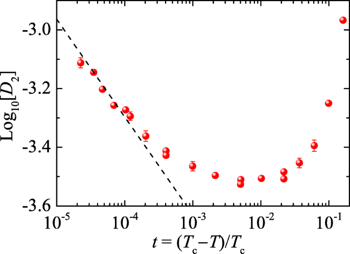
Second sound diffusivity D2, in units of cm2/s, as a function of the reduced temperature t=(Tc−T)/Tc. The experimental data (circles) are from Mehrotra and Ahlers in 1983, measured from the resonance line width of cw cavities [40]. The dashed line illustrates the critical behavior D2∝t−ν/2 near the superfluid lambda transition, with a critical exponent ν≃2/3
Historically, the measurement of second sound attenuation in superfluid helium plays a crucial role to establish the celebrated dynamic scaling theory of superfluid phase transition [41, 42]. By extending the static scaling ideas that involves the coherent length ξ(T)∝(Tc−T)−ν, where ν≃2/3 is the critical exponent, Ferrell and his co-workers stated that the dynamics near the phase transition is governed by a characteristic frequency ω∗=c2/ξ. As the second sound velocity vanishes like c2∝(Tc−T)ν/2 close to the transition, both the sound diffusivity D2 and the thermal conductivity κ then would diverge as |Tc−T|−ν/2. This critical divergence can be clearly seen in Fig. 2, where the critical scaling law |t|−ν/2 is illustrated by the dashed line. The data seems to deviate from the critical divergence at the reduced temperature \(t\gtrsim 5\times 10^{-4}\), strongly indicating the existence of a quantum critical regime at |t|<5×10⁻⁴ or |Tc−T|<1 mK.
It is worth noting that a minimum second sound diffusivity (D2)min≃10−3.54 cm2/s appears at |t|∼10−2 [43]. In terms of \(\hbar /m\simeq 1.59\times 10^{-4}\) cm2/s for the mass of helium atoms, we find that:
A similar minimum occurs in the thermal diffusivity DT at the same temperature range |t|∼10−2 just above the superfluid transition [43]: \((D_{T})_{\text {min}}\simeq 1.5\hbar /m\).
Hydrodynamic regime vs quantum criticality
Landau’s two-fluid hydrodynamic equations are applicable in the limits of long wavelength and low frequency [39], i.e., kξ≪1 and ωτ≪1, where τ is a characteristic collision time.
Very close to the superfluid lambda transition, the former condition kξ≪1 necessarily breaks down, due to the divergent correlation length ξ→∞ [42]. A reasonable estimate of ξ in the superfluid phase is given by [42], ξ∼r0|t|−ν, where r0≃2.22 Å is the mean distance between two helium atoms. This seems to impose a stringent restriction for the use of neutron scattering, since the transferred momentum k in the neutron-scattering experiment is typically larger than 0.1 Å −1 [44], and hence, the hydrodynamic regime is difficult to reach. Brillouin light scattering can instead be used to measure the density correlation function (i.e., dynamical structure factor) in the hydrodynamic regime [45], with a momentum kr0∼0.004 or kξ≃0.004|t|−ν. However, one may hardly reach the quantum critical regime at |t|<5×10⁻⁴, as suggested by the data in Fig. 2. This is consistent with the observation in the Brillouin light scattering experiment [45] that, below the superfluid transition, the second sound attenuation starts to saturate at |Tc−T|<1 mK.
On the other hand, the latter hydrodynamic condition ωτ≪1 becomes more difficult to satisfy at very low temperature. In the measurement of first sound attenuation, one typically observes a maximum at T∼0.4Tc≃0.9 K [46], due to the transition from the hydrodynamic regime to the collisionless regime.
Second sound in unitary Fermi gas: earlier theoretical treatments
Let us now look back to year 2005. At that time, Fermi superfluidity near a Feshbach resonance has been unambiguously verified, by measuring nonzero condensate fraction [16, 17] and by observing vortex lattice [18]. Yet, there was no trace for the most important second sound, presumably due to two technical difficulties. On the one hand, the thermodynamic functions or equations of state of a unitary Fermi gas were less known. In particular, the superfluid density had only been calculated using the mean-field Bardeen-Cooper-Schrieffer (BCS) theory, which is not so accurate. On the other hand, a unitary Fermi gas had have to be confined in a harmonic trap. While zero-temperature first sound such as the breathing mode of a trapped unitary Fermi gas was theoretically discussed [9–11] and experimentally explored in detail [6–8], at finite temperature both first and second sound modes in a harmonic trap were not considered.
The first problem was partly solved with the development of strong-coupling diagrammatic theories at the BEC-BCS crossover [20, 47]. In particular, the superfluid density has been calculated by the Gaussian pair fluctuation (GPF) theory [19], in which strong bosonic pair-fluctuations at the Gaussian level are taken into account on top of the standard BCS mean field theory (see also the simplified treatment of the bosonic degree of freedom in Ref. [48] and Ref. [49]). As shown in Fig. 3, the GPF theory predicts a larger superfluid density than the BCS mean-field theory. Compared with superfluid helium, unitary Fermi gas turns out to have a smaller superfluid fraction. It is worth noting that, for the superfluid density of a unitary Fermi gas, the GPF result remains as the best theoretical prediction so far [14], since ab initio quantum Monto Carlo simulation is still not available towards the meaningful thermodynamic limit.
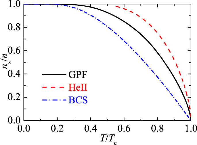
The superfluid fraction of a unitary Fermi gas, predicted by the Gaussian pair fluctuation (GPF) theory (black solid line) and mean-field BCS theory (blue dot-dashed line). For comparison, the superfluid fraction of superfluid helium is also shown by a red dashed line. Note that, the GPF theory predicts a spurious bend-back structure near the superfluid transition [19]. This unphysical behavior has been rectified [14], by extrapolating the reliable results below Tc with the correct critical scaling behavior ns/n∝(1−T/Tc)−ν, with ν≃2/3. Here, the critical temperature of a unitary Fermi gas is Tc≃0.17TF, as determined experimentally. The Fermi temperature \(T_{F}=\varepsilon _{F}/k_{B}=\hbar ^{2}k_{F}^{2}/(2mk_{B})\) and the Fermi wavevector kF=(3π2n)1/3 at density n
The GPF theory also predicts reasonably accurate thermodynamic functions for unitary Fermi gas [20, 50]. By applying the dissipationless two-fluid hydrodynamic equations, it is then straightforward to calculate the first and second sound velocities in the unitary limit [15], as reported in Fig. 4. Remarkably, the temperature dependence of second sound velocity in unitary Fermi gas is qualitatively similar to that of superfluid helium, in spite of the entirely different statistics of the two systems. At low temperatures, we may attribute the similarity to gapless phonon excitations, which are the dominant quasiparticles of both systems. At temperatures close to the superfluid transition, fermionic gapped single-particle excitations become important in unitary Fermi gas. It seems reasonable to argue that these single-particle excitations may play the same role as rotons in superfluid helium, which are also gapped, single-particle-like excitations.
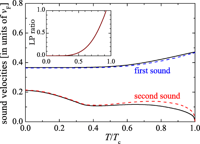
First and second sound velocities of a uniform Fermi gas at unitarity (solid lines), predicted by the GPF theory. The units of the velocity is \(v_{F}=\hbar k_{F}/m\). The uncoupled first and second sound velocities given by vS and v are shown as dashed and dotted lines, respectively. The inset shows the Landau-Placzek ratio as a function of T/Tc. From Ref. [15]
Despite the similar temperature dependence in second sound velocity, there is an important difference between unitary Fermi gas and superfluid helium. As shown in the inset of Fig. 4, unlike superfluid helium the LP ratio of a unitary Fermi gas can be very significant already at T∼0.6Tc, suggesting a strong coupling between first and second sound. As a result, we should be able to observe the temperature wave of second sound from the density response. This solves a potential detection problem, since we can hardly have a local thermometer with cold atoms. The density response, however, is easy to measure, by using Bragg scattering technique [51].
A significant LP ratio also implies that the second sound velocity deviates from v. By solving Eq. (5), we find that the expansion [52]:
in terms of the parameter \(x\equiv (v^{2}c_{V})/(v_{S}^{2}c_{P})\), which is very small in the temperature region of interest (i.e., T>0.6Tc). Thus, the second sound velocity can be well approximated by:
Second sound in a harmonic trap
The second problem related to the harmonic trapping potential Vext(r) was solved by Griffin and his colleagues, with a reformulation of Landau’s dissipationless two-fluid hydrodynamic equations in a variational form [13–15]. This reformulation is crucial, since the brute-force solution of Landau’s two-fluid equations turns out to be difficult [12, 53].
By introducing the displacement fields us and un through vs(r,t)=∂us(r,t)/∂t and vn(r,t)=∂un(r,t)/∂t, they found that the solution of hydrodynamic modes with frequency ω (i.e., us(r,t)=us(r)e−iωt and un(r,t)=un(r)e−iωt) can be derived by minimizing the variational expression [13]:
where the superfluid density ns(r), the normal density nn(r), and the various equilibrium thermodynamic variables (∂μ/∂n)s,(∂T/∂n)s and (∂T/∂s)n are position-dependent due to the harmonic trap Vext(r), and their spatial dependence can be calculated within the standard local density approximation. The action Eq. (13) includes the kinetic energy terms due to the displacement fields of the superfluid component (us(r)) and of the normal component (un(r)), and the potential energy terms arising from the density fluctuation δn and entropy fluctuation δs, which are respectively given by:
The minimization of the action can be easily carried out by applying a variational polynomial Ansatz for the displacement fields [15].
The variational expression of the two-fluid hydrodynamic theory is very useful to understand the decoupled first and sound modes in traps. For the pure in-phase mode of first sound, we can insert us(r)=un(r)=u(1)(r) into the action Eq. (13) and take the variation with respect to u(1)(r). It is straightforward to show that:
which without the harmonic trap (Vext=0) gives the plane wave solution ∝eik·r with dispersion ω1=vSk. For the pure out-of-phase mode of second sound, the density fluctuation δn=0, and we then inset \(n_{s}\mathbf {u}_{s}^{(2)}(\mathbf {r})=-n_{n}\mathbf {u}_{n}^{(2)}(\mathbf {r})\) into Eq. (13) to obtain:
In the absence of the trapping potential, it gives rise to the plane wave solution with dispersion ω2=vk, as anticipated.
The coupled first sound and second sound in an isotropic harmonic trap \(V_{ext}(r)=m\omega _{0}^{2}r^{2}/2\) have been solved for the compressional modes with angular momentum l=0, by applying the following variational Ansatz [15]:
with N variational parameters {as,j,an,j}. Figure 5a shows the mode frequencies as a function of the temperature, obtained with N=8, which is large enough to have convergent results for the variation calculations. Also shown are the frequencies of the decoupled first sound [ ω1(n), blue dashed lines] and second sound [ ω2(n), red dotted lines] modes given by Eqs. (16) and (17), respectively, where n=0,1,2,⋯ is the number of radial nodes. First sound appears to be the “horizontal” branches, with mode frequency decreases with increasing temperature. In contrast, at T>0.4Tc the mode frequency of second sound increases rapidly with temperature and becomes divergent close to the superfluid transition, i.e., ω2∝(1−T/Tc)(ν−1)/2, where ν≃2/3 is the critical exponent. This peculiar divergence is found to be related to the critical behavior of superfluid density [15].
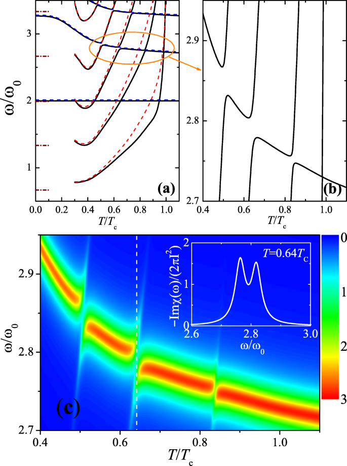
a Two-fluid modes of a unitary Fermi gas in an isotropic harmonic trap. The full solutions of the two-fluid equations are given by the solid lines. The first sound modes (blue dashed lines) given by Eq. (16) are shown along with the second sound modes (red dotted lines) given by Eq. (17). The dashed lines at T=0 show the analytic results for the second sound frequency. b A blow-up of part of the left panel showing the hybridization between second sound and the n=1 first sound mode. c The two-dimensional contour plot of the density response Imχ(ω) in the vicinity of the n=1 first sound mode. The delta functions in Imχ(ω) have been broadened by 0.02ω0 for visibility. The inset shows a double peak structure at the hybridization point T≃0.64Tc. Adapted from Ref. [15]
To experimentally probe the second sound branches, the authors proposed to use Bragg scattering to measure the density response [15], thanks to the significant LP ratio of unitary Fermi gas and hence the strong coupling between first second and second sound. This is evident in Fig. 5b from the avoided crossings and hybridizations, which mean that second sound will manifest itself in the density response at the crossing points. By adding a density perturbation of the form δV∝f(r)e−iωt to the variational action Eq. (13), it is easy to derive the density response function \(\chi (\omega)=\int d\mathbf {r}f(\mathbf {r})\delta n(\mathbf {r})\), with imaginary part (Z1+Z2=1)
near a crossing point with mode frequencies \(\tilde {\omega }_{1}\) and \(\tilde {\omega }_{2}\). The weights Z1 and Z2 becomes equal at the crossing point. Fig. 5c clearly shows the bimodal structure in the vicinity of hybridization between the n=1 first sound mode and second sound. The inset highlights the hybridization point at T≃0.64Tc, where the first sound and second sound contribute equally to the density response (i.e., Z1∼Z2). The frequency splitting Δω∼0.06ω0 between the two peaks is large enough to be resolved in experiments. On the other hand, for the low-lying collective modes in harmonic traps, both viscous damping and thermal damping are supposed to be small, so the double peak structure shown in the inset could be robust.
Second sound propagation in a uniform system
To better understand the second sound of a unitary Fermi gas, Griffin and his colleagues also discussed in detail the sound propagation in the uniform configuration [52]. By setting Vext=0 and adding a density perturbation with a given momentum k, i.e., δV∝ei(k·r−ωt), to the variation action, it is straightforward to derive the density response function [52]:
with imaginary part (ω>0):
where \(Z_{1}\equiv (c_{1}^{2}-v^{2})/(c_{1}^{2}-c_{2}^{2})\) and Z2=1−Z1. By defining \(W_{1}=Z_{1}/c_{1}^{2}\) and \(W_{2}=Z_{2}/c_{2}^{2}\), we find that the relative weight of second sound and first sound in the Bragg scattering is given by [52]:
For unitary Fermi gas, the ratio W2/W1 is roughly equal to the LP ratio εLP, as shown in Fig. 6a. Therefore, although the LP ratio is significant close to the superfluid transition, the second sound signal in the Bragg scattering measurement would be still much weaker than the first sound signal, due to the additional reduction factor c2/c1, which is less than 0.3 in the temperature region of interest. The weak second sound signal in the density response −Imχ is explicitly illustrated in Fig. 6b.
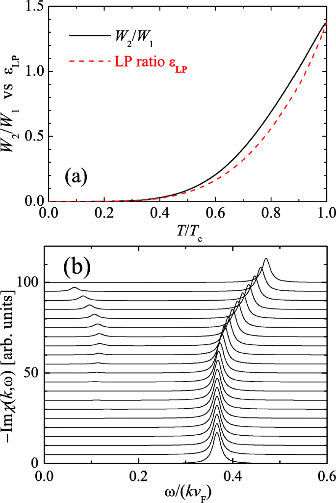
a Comparison between the ratio of the second and first sound amplitudes in the dynamic structure factor (W2/W1) and the Landau–Placzek ratio εLP in a unitary Fermi gas. b The imaginary part of the density response function at k=0.1kF and at different temperatures (each temperature is offset). The temperature is increased from zero to Tc, in steps of 0.05Tc. For clarity, the delta functions in Eq. (21) are plotted as Lorentzians with a width 0.01kvF. Adapted from Ref. [52]
Unitary Fermi gas vs weakly interacting Bose gas
The similarity of second sound in unitary Fermi gas and superfluid helium strongly indicates that the qualitative behavior of second sound is insensitive to the statistics of underlying particles. Instead, the inter-particle interaction strength may play an important role. To confirm such an idea, Griffin and his colleagues investigated the sound propagation in interacting molecular Bose gas of tightly bound Cooper pairs of mass mB=2m with tunable interaction strength [52], as shown in Fig. 7. In the BEC limit, the molecular scattering length aB≃0.6a [54] and the density nB=n/2. In their calculations, the thermodynamic functions in Landau’s two-fluid hydrodynamic equations are calculated by using the standard Hartree-Fock-Bogoliubov-Popov theory at finite temperature, and the superfluid density is approximated by the condensate density, i.e., ns(T)≃nc(T)≤nB.
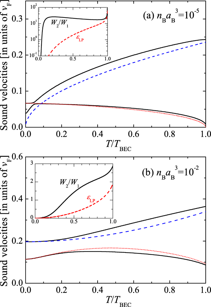
First and second sound velocities in an interacting molecular Bose gas with gas parameter \(n_{B}a_{B}^{3}=10^{-5}\) (a) and \(n_{B}a_{B}^{3}=10^{-2}\) (b). In a, the blue dashed and red dotted lines show cHF(T) and cB(T); while in b, they are respectively the approximate velocities c1=vS and \(c_{2}=v/\sqrt {c_{P}/c_{V}}\). The two inset show the LP ratio εLP (red dashed line) and the weight ratio W2/W1 (black solid line). Adapted from Ref. [52]
For a weakly interacting Bose gas with gas parameter na3=10−5 [Fig. 7a], first sound and second sound show an interesting hybridization at very low temperature [55, 56]. This hybridization is due to the large compressibility of the weakly interacting Bose gas, which leads to a large LP ratio εLP or W2/W1, as shown in the inset. It is natural to identify the upper and lower branches of sound velocities as first sound and second sound. Below the hybridization point, the first sound velocity approaches the Bogoliubov phonon velocity [52, 56]:
and first sound corresponds to an oscillation of the condensate component. Above the hybridization point, the role of first sound and second sound exchanges. It is second sound that propagates with the phonon velocity cB. Consequently, second sound in dilute molecular Bose gas (above the hybridization temperature) is essentially an oscillation of the condensate at all temperatures, with a static thermal cloud. In contrast, first sound describes an oscillation of the thermal cloud in the presence of a stationary condensate. In the Hartree-Fock approximation, its velocity is given by [56]:
where \(g_{n}(z)=\sum _{l=1}^{\infty }z^{l}/l^{n}\) is the usual Bose-Einstein function and nn(T)≃n−nc(T) is the density of the normal-fluid component.
The situation completely changes when we tune the gas parameter to the strongly interacting regime (i.e., \(n_{B}a_{B}^{3}=0.01\)) [52]. As shown in Fig. 7b, the velocities of first and second sound never become degenerate (cross), and thus, the hybridization found in Fig. 7a does not occur. In this strongly interacting Bose superfluid, we also show the approximate velocities of c1=vS and \(c_{2}=v/\sqrt {c_{P}/c_{V}}\), given by the leading term of Eqs. (10) and (11). These approximate values give a reasonable first order approximation to the full solutions of the first and second sound velocities. Overall, we see that the qualitative behavior of sound velocities in the strongly interacting Bose superfluid is close to that of a unitary Fermi gas reported in Fig. 4.
Second sound in unitary Fermi gas: the first observation
The analysis of hydrodynamic modes in an isotropic harmonic trap is difficult to experimentally verify, since in experiments the trapping potential is general axially symmetric. To overcome this problem, Stringari and his colleagues suggested using a highly elongated cigar-like trap and derived reduced one-dimensional (1D) Landau’s two-fluid hydrodynamic equations [21, 22]. Their brilliant idea on quasi-1D hydrodynamic modes eventually leads to the first experimental observation of the second sound propagation in 2013 [23].
Quasi-1D Landau’s two-fluid hydrodynamic equations
Let us consider that a unitary Fermi gas flows through a highly-elongated trapping potential \(V_{\text {ext}}(\mathbf {r})=m(\omega _{\perp }^{2}x^{2}+\omega _{\perp }^{2}y^{2}+\omega _{z}^{2}z^{2})/2\) with trapping frequency ω⊥≫ωz. This case may be compared with the flow of superfluid helium through a narrow capillary tube [39]. If the wavelength of the helium flow is comparable to or greater than the diameter of the tube, the normal-fluid component becomes stationary and sticks to the hard wall of the tube due to its viscosity. The sound propagation is then all carried by the superfluid component, forming the so-called fourth sound [58]. In the current situation of a soft harmonic trap, the normal-fluid component will keep moving. However, the viscosity may be sufficiently large to ensure that the normal velocity vn(z) does not depend on the radial coordinates (x or y); otherwise, the sound propagation will involve excitations costing large energy at the order of ω⊥ [21]. Similarly, a large thermal conductivity may make the temperature uniformly distributed in the radial direction [21].
Due to the independence of the dynamic variables on the radial coordinates, we may perform the integration over the radial degree of freedom in all the equilibrium thermodynamic functions and deduce the quasi-1D thermodynamics. For example, we can define the reduced 1D superfluid density \(n_{s1}(z)\equiv \int dxdyn_{s}(\mathbf {r})\), normal density \(n_{n1}(z)\equiv \int dxdyn_{n}(\mathbf {r})\), and entropy \(s_{1}(z)\equiv \int dxdys(\mathbf {r})\). By introducing the displacement fields us(z) and un(z), we write down the variational action [22, 59]:
where n(z)=ns1(z)+nn1(z) is the reduced 1D total density, and δn(z)≡−∂(ns1us+nn1un)/∂z and δs(z)≡−∂(s1un)/∂z are the density and entropy fluctuations, respectively. The effect of the weak axial trapping potential \(V_{\text {ext}}(z)=m\omega _{z}^{2}z^{2}/2\) now enters Eq. (25) via the z-dependence of the equilibrium thermodynamic variables, within the local density approximation.
To examine the reduced 1D two-fluid hydrodynamics, low-lying first sound modes in elongated harmonic traps were measured by the Innsbruck group [57]. First sound is the pure-phase mode with us(z)=un(z)=u(1)(z). The minimization of the action \(\mathcal {S}_{1D}\) with respect to u(1)(z) yields the following equation for the first sound mode [22, 57]:
where \(P_{1}\equiv \int dxdyP(\mathbf {r})\) is the reduced 1D pressure. It is easy to find the solution of Eq. (26), by again using a polynomial Ansatz [22, 57]:
with integer values of k. The lowest axial breathing mode has a frequency \(\omega _{k=1}=\sqrt {12/5}\omega _{z}\), which is temperature independent due to the scaling invariance of the unitary Fermi gas [60]. Experimentally, therefore, it is useful to measure the k=2 mode or k=3 mode, which shows the interaction effects through the temperature dependence of the equation of state (EoS). The theoretical prediction on the frequency of the k=2 first sound mode as a function of temperature is presented in Fig. 8. Indeed, by comparing the green solid line (with a unitary gas EoS measured by the MIT group [61]) and the green dashed line (with an ideal Fermi gas EoS), we can see clearly the interaction effect. The first sound mode frequency changes smoothly across the superfluid phase transition (as indicated by the red dash-dotted vertical line). The experimental data agree reasonably well with the theoretical prediction based on the reduced 1D two-fluid hydrodynamic equations. This provides a strong support for the applicability of the reduced 1D description.
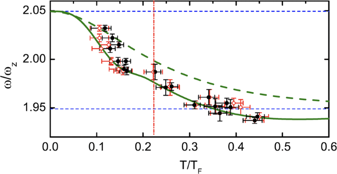
Comparison between experimental (symbols) and theoretical (green lines) first sound frequencies of the k=2 mode. The different symbols correspond to different ways of determining temperature. In theoretical calculations, both the equations of state of a unitary Fermi gas (green solid line) and of an ideal Fermi gas (green dashed line) are used. The two thin blue horizontal dashed lines mark the zero-temperature superfluid limit (\(\omega /\omega _{z}=\sqrt {21/5}\)) and the classical hydrodynamic limit (\(\omega /\omega _{z}=\sqrt {19/5}\)), respectively. The red dash-dotted vertical line indicates the critical temperature in traps Tc≃0.223(15)TF. Adapted from Ref. [57]
We note that, the full minimization of the variational action with respect to us(z) and un(z) has also been performed [59]. The coupling between first sound and second sound only leads to a very small correction to the k=2 mode frequency ωk=2.
First observation of second sound propagation
The Innsbruck group then considered the second sound propagation in an elongated harmonic trap with trapping frequency ω⊥=2π×539(2) Hz and ωz=2π×22.46(7) Hz [23]. For sound waves with excitation energy ω⊥>ω≫ωz, the discreteness in energy due to the weak confining potential \(V_{ext}(z)=m\omega _{z}^{2}z^{2}/2\) is not important. The sound waves propagate with a local velocity that slowly varies across the whole trap. By setting a plane wave solution in the form of ei(kz−ωt), it is straightforward to derive the second sound velocity [22]:
where the reduced 1D entropy per particle \(\bar {s}_{1}\) and the reduced 1D specific heat per particle at constant pressure \(\bar {c}_{P1}\) can be calculated by using the known EoS of a unitary Fermi gas, as measured by the MIT group in 2012 [61]. If the local second sound velocity c2(z) is measured, from the above expression one can then straightforward to determine the local reduced 1D superfluid fraction [ns1/n1](z) as a function of the local reduced temperature \(T/T_{F}^{1D}\), where \(T_{F}^{1D}\equiv (15\pi /8)^{2/5}(\hbar \omega _{\perp })^{4/5}[\hbar ^{2}n_{1}^{2}/(2m)]^{1/5}/k_{B}\) is a natural definition for Fermi temperature in highly elongated harmonic traps. Consequently, the superfluid fraction ns/n as a function of the reduced temperature T/TF can be reconstructed, thanks to the universal thermodynamic functions in the unitary limit [50, 60].
To excite the second sound, the Innsbruck group used the same heating strategy as in the superfluid helium. As shown in Fig. 9a, a weak power-modulated repulsive laser beam intersects the cigar-shape Fermi cloud in the middle. A burst with eight sinusoidal oscillations in a few milliseconds then excites a second sound wave, whose propagation with time is presented in Fig. 9(c). Two local density dips are clearly visible within the superfluid region (as enclosed by the two vertical dashed lines). The dips move very slowly when they approach the superfluid boundary and finally disappear. The fact that this sound wave cannot propagate in the non-superfluid region is a fingerprint characteristic of the second sound.
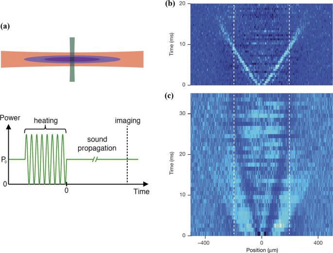
a A second sound wave is excited by a weak, power-modulated repulsive laser beam (green) that perpendicularly intersects the cigar-like Fermi cloud (purple) with a total N=3×1056Li atoms. The short power-modulation burst contains eight sinusoidal oscillations (i.e., heating) in 4.5 ms. The sinusoidal oscillations are absent if a first sound wave is excited. b, c Normalized differential axial density profiles, measured for variable delay times after the excitation, show the propagation of first sound (local density increase, bright) and second sound (local decrease, dark). The temperature of the Fermi cloud is T=0.135(10)TF, where \(T_{F}=\hbar (3N\omega _{\perp }^{2}\omega _{z})^{1/3}\) is the Fermi temperature in traps. The vertical dashed lines indicate the axial region where superfluid is expected to exist (i.e., |z|<190μm). Adapted from Ref. [23]
In contrast, a first sound wave can be excited without the heating sinusoidal oscillations, as shown in Fig. 9b. The first sound manifests itself as two local density peaks. They move much faster than the second sound dips in Fig. 9c. Obviously, they can penetrate through the superfluid boundary and propagate freely into the non-superfluid region, as anticipated.
The first and second velocities can be easily extracted from the time evolution of the peak position (for first sound) and the dip position (for second sound). For example, by fitting the pulse (peak or dip) position as function of time with a third-order polynomial, the sound velocity can be straightforwardly determined by taking the time derivative of the fitting curve. The results are shown in Fig. 10a by solid lines. Alternatively, the time derivative can be taken by analyzing the subsets of nine adjacent profiles, which leads to the data points (symbols) in the figure. For the first sound velocity, the experimental data agree well with the theoretical prediction \(c_{1}=\sqrt {7P_{1}/(5mn_{1})}\), which can be easily derived by using Eq. (26) in the absence of the weak confining potential (i.e., ωz=0).
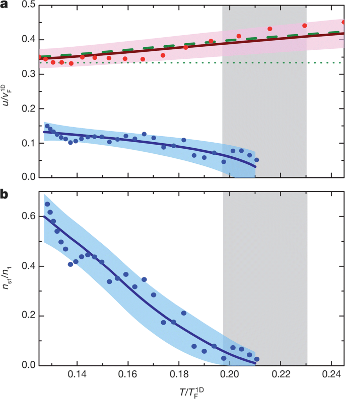
a The measured first and second sound velocities as a function of the reduced temperature \(T/T_{F}^{1D}\). The solid lines and symbols are experimental results from different methods of taking the time derivative of the pulse position of sound wave (i.e., through a polynomial fit or through analyzing subsets of nine adjacent profiles). The green dashed line for first sound velocity is the theoretical prediction \(c_{1}=\sqrt {7P_{1}/(5mn_{1})}\). b Temperature dependence of the reduced 1D superfluid fraction ns1/n1. The grey-shaded area indicates the uncertainty range of the superfluid phase transition. From Ref. [23]
From the second sound velocity, it is straightforward to determine the reduced 1D superfluid fraction ns1/n1, by using Eq. (28). This unknown quantity is presented in Fig. 10b. It decreases monotonically with increasing temperature and vanishes in the uncertainty range of the superfluid phase transition.
The reconstruction of the most important uniform superfluid fraction ns/n from ns1/n1 is also straightforward [23]. The result is shown in Fig. 11, with the uncertainty indicated by the blue shaded area. It is interesting to see that the measured superfluid fraction of unitary Fermi gas follows closely that of superfluid helium (green solid line). However, the uncertainty of the data points seems to be too large to make a convincing conclusion. Nevertheless, the superfluid fractions of both unitary Fermi gas and superfluid helium are much larger than the condensate fraction of an ideal Bose gas (red dashed line).
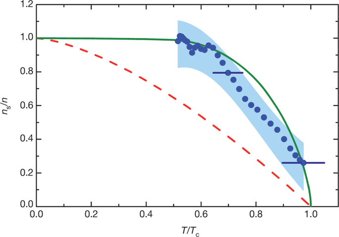
The reconstructed superfluid fraction of a uniform unitary Fermi gas (symbols) as a function of T/Tc, with uncertainty range indicated by shaded region. For comparison, the superfluid fraction of superfluid helium (green line) and the condensate fraction of an ideal Bose gas 1−(T/Tc)3/2 (red dashed line) are also shown. From Ref. [23]
Second sound propagation at the BEC-BCS crossover
The landmark experiment by the Innsbruck group focused on the unitary limit. Recently, the same-type measurement has been carried out at the whole BEC-BCS crossover by Hoffmann and his colleagues at Ulm University [63]. Their result of the second sound velocity as a function of the interaction parameter 1/(kFa) is presented in Fig. 12. The temperature varies in the range T/Tc=0.66−0.84. In this temperature range, the second sound velocity shows a pronounced maximum slightly above the unitary limit 1/(kFa)∼0.4. Overall, the measured second sound velocity agrees qualitatively well with an earlier theoretical calculation (blue dash-dotted line) based on the mean-field superfluid density and thermodynamic functions [62]. A refined theoretical analysis beyond the mean-field treatment would be useful to better understand the experimental data at the BEC-BCS crossover.
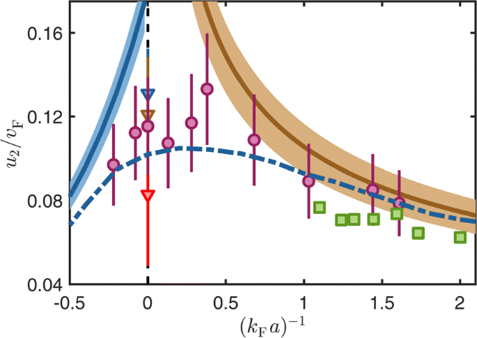
The purple circles are the measured data from the Ulm experiment for temperatures in the range T/Tc=0.66−0.84. The brown and blue solid line show analytic predictions for the BEC and BCS regime at T=0.75Tc, respectively. The blue dash-dotted line shows an earlier theoretical prediction of second sound at the crossover at T/Tc=0.75 [62]. The green squares are results of numerical c-field simulations. For comparison, the second sound velocities of a unitary Fermi gas measured by the Innsbruck group [23] at the temperatures T/Tc=0.65 (blue triangle), T/Tc=0.75 (brown triangle), and T/Tc=0.85 (red triangle) are also shown. From Ref. [63]
Second sound in unitary Fermi gas: the measurement of sound attenuation
It is a milestone to observe the second sound of unitary Fermi gas in highly elongated harmonic traps [23]. However, the trapping potential seems to be very unfriendly for the purpose of performing precise measurements. On the one hand, the variation of local density along the weakly confined direction brings a relatively large uncertainty on the measured 1D sound velocities and hence on the extracted 1D superfluid fraction, as we already see from Fig. 10. On the other hand, the reduced 1D Landau’s two-fluid hydrodynamic equations are dissipationless due to the dimensional reduction [21, 22]. As a result, there is no theoretical guidance on how to extract the important second sound attenuation and the related transport coefficients such as shear viscosity η and thermal conductivity κ, if the damping of 1D sound propagation is measured.
This serious technical difficulty could be overcome, owing to the experimental realization of a box-like trapping potential and consequently a homogeneous interacting Fermi or Bose gas [24, 25]. Indeed, the first sound attenuation of a homogeneous unitary Fermi gas was recently measured by Patel and his colleagues at Massachusetts Institute of Technology (MIT) [64]. The measurement of second sound and its attenuation has also been attempted at MIT, by setting up a local cold-atom thermometry to measure the temperature wave. However, this is difficult. It turns out that a direct and more efficient way is to measure again the density signal of second sound thanks to the appreciable LP ratio of unitary Fermi gas. A high-resolution Bragg spectroscopy was set up for this purpose by the USTC group [33]. The second sound attenuation was then successfully measured [33].
Hydrodynamic density response function
Before we discuss the USTC experiment on the second sound attenuation, it is useful to briefly describe the density response function in Landau’s two-fluid hydrodynamic theory. Its expression was first derived by Hohenberg and Martin in their seminal work [65] and takes the following form for an isotropic superfluid (such that χ(k,ω)=χ(k,ω)):
where the damping rate or sound attenuation of the response is characterized by three diffusion coefficients D1,D2, and Ds, as determined by solving the coupled equations:
Here, ρ=mn=m(ns+nn) is the total mass density, and we do not include the various second viscosities ζi (i=1,2,3,4), since for a unitary Fermi gas only ζ3 can be non-zero but its value could be insignificant to have sizable contribution. In the absence of the diffusivities D1,D2, and Ds, the hydrodynamic density response Eq. (29) reduces to the familiar dissipationless form in Eq. (20). There are two sources for dissipation that is responsible for the sound attenuation. One is the viscous damping stemming from the diffusion of momentum, characterized by the shear viscosity η (and various second viscosities that we neglect). Another is the thermal damping caused by diffusion of heat, given by the thermal conductivity κ. The relative contribution of these two sources can be quantified by a dimensionless Prandtl number:
It is interesting to note that, over the last two decades, the measurements of both shear viscosity η and thermal conductivity κ of strongly interacting unitary Fermi gas have received increasing attention from a diverse fields of physics. For shear viscosity η, it is anticipated that the unitary Fermi gas may behave like a perfect fluid, with viscosity-to-entropy ratio η/s close to a universal lower-bound 1/(4πkB) conjectured by Kovtun, Son, and Starinets (KSS) [66]. The measurement of thermal conductivity κ is equally important. From the AdS/CFT correspondence, a holographic conformal nonrelativistic fluid has a Prandtl number Pr=1 [67]. Therefore, it would be interesting to check whether a unitary Fermi gas can be treated as a holographic dual near the superfluid phase transition, where the conformal invariance might be satisfied. We also note that, the shear viscosity of unitary Fermi gas has been measured at North Carolina State University (NCSU) from the anisotropic expansion of the Fermi cloud for a wide temperature window [28], ranging from ∼TF down to far below the transition temperature. Less is known about the thermal conductivity, except the high-temperature classical regime [30], where \(\kappa _{\text {cl}}=(n\hbar k_{B}/m)(675\sqrt {2}\pi ^{3/2}/512)(T/T_{F})^{3/2}\).
As in the dissipationless case, it is intuitive to separate the first and second sound contributions to the density response function Eq. (29). By ignoring the high-order terms of the small parameter εLP(c2/c1)2, we find that [33]:
where
with the thermal diffusivity DT≡κ/(ρcP). It is easy to see that, above the superfluid transition (c1=vS and D2=DT), the second sound turns into a thermally diffusive mode, with a contribution [32]:
which peaks around the zero frequency ω=0.
Second sound attenuation measurement
In the USTC experiment [33], a novel high-resolution Bragg spectroscopy has been developed to directly probe the density signals from both first sound and second sound. As shown in Fig 13a, a high-density population-balanced Fermi mixture at the Feshbach resonance is realized in a box trap with about 1076Li atoms, much denser than earlier experiments where the number of atoms is typically in the range of 104−106. This state-of-the-art preparation of Fermi superfluid typically yields a high density n≃1.56×1013 cm−3, a large Fermi wavenumber kF=(3π2n)1/3≃2π×1.23 μm−1, and also a large Fermi energy \(E_{F}\simeq 2\pi \hbar \times 50\) kHz. By further applying a pair of coherent 741-nm laser beams with frequency difference ω (see Fig. 13(b)), a moving-lattice potential is formed to create density fluctuations. The angle between two lattice lasers can be finely tuned to give rise to a very small Bragg momentum k=2π×0.071 μm−1≃0.058 kF. Therefore, if we estimate the correlation length \(\xi \sim k_{F}^{-1}|t|^{-\nu }\) as in superfluid helium and optimistically take the criterion kξ<1 for the hydrodynamic regime, the hydrodynamic description for the density response function Eq. (29) would be applicable over a wide temperature range unless very close to the superfluid transition, i.e., |t|<0.014 or |T−Tc|<0.002 TF. After applying the moving lattice potential with strength V0 for 3 milliseconds, a steady-state density fluctuation can be measured, as reported in Fig. 13c for first sound and Fig. 13d for second sound at T=0.84Tc. The density fluctuation should take the form, δn(z,t)=|χ(k,ω)|V0 sin[kz−ωt+φ(k,ω)], from which the modulus of the density response function |χ(k,ω)| is determined.
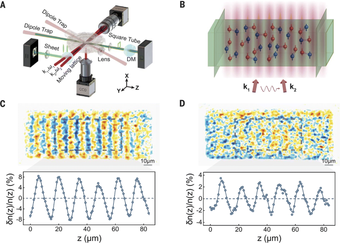
a The experimental setup: a box trap consists of a square tube and two sheets of laser beams. b A pair of 741-nm laser beams with wave numbers (k1=k2=kL) and frequencies (ω1,ω2) intersect on the homogeneous unitary Fermi gas with a small angle, producing a one-dimensional moving-lattice potential. c, d First and second sound waves. The upper panels show two typical single-shot images of unitary superfluid at T=0.84Tc, taken at the frequencies ω=ω1−ω2=2.1 kHz and 0.3 kHz, respectively. To clearly show the density waves along the longitudinal z-axis, we have taken the difference with respect to a reference image at ω=1 MHz. Further integration of the difference along the two transverse directions in the region of interest, as marked by the dashed box, reveals a normalized density fluctuation δn/n propagating along the z-axis, as shown in the low panels. From Ref. [33]
There are two key technical advantages of the developed high-resolution Bragg spectroscopy at USTC. First, the modulus |χ(k,ω)| is directly obtained from the integration of |δn/n| as a function of ω, contrasted with Im[χ(k,ω)] from the out-of-phase density response in other experiments [34, 64]. This avoids potential errors due to the phase synchronization. On the other hand, more importantly, the steady-state density response removes a large instrumental spectral broadening ∼0.1EF due to a finite Bragg pulse duration in the conventional Bragg spectroscopy [68, 69] (as well as in the inelastic neutron scattering experiments of superfluid helium [44]). Both advantages, together with the large Fermi energy, makes it possible to directly probe the second sound.
The density response spectra |χ(k,ω)| over a wide range of temperature T⊆[0.42,1.04]Tc have been systematically measured in the experiment. The representative spectra from 0.75 Tc to 0.94 Tc are reported in Fig. 14. A second sound peak can be clearly identified at low-frequency ω<0.01EF, in addition to a high-frequency first-sound peak at ω∼0.045EF. The simultaneous appearance of both first sound and second sound signals is a unambiguous proof of Landau’s two-fluid description of the density response in the long-wavelength and low-energy hydrodynamic regime. Indeed, the measured density response can be well fitted by using Eq. (14), with various sound velocities (c1,c2 and v) and sound diffusivities (D1,D2 and Ds) as six fitting parameters.
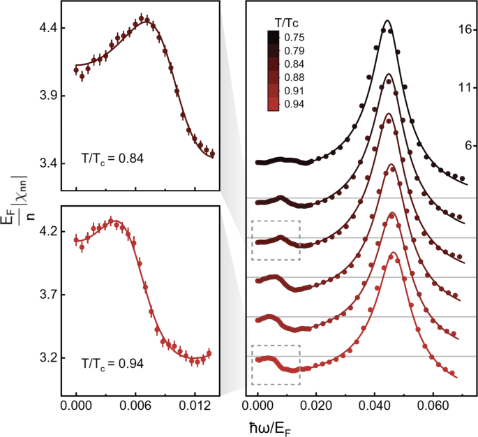
The second sound signal is particularly evident at T∼0.8−0.9Tc, as highlighted in the left panel of Fig. 14. It is worth noting that, the peak does not show a symmetric Lorentzian line-shape as we anticipate for a propagating sound, since it is the modulus |χ(k,ω)| being plotted, instead of Im[χ(k,ω)]. At zero frequency, the density response function is given by the compressibility sum-rule [44, 52]:
and therefore is non-zero. To further characterize the second sound contribution in the density response, Im[χ(k,ω)] can be reconstructed by using the six fitting parameters. A well-defined propagating second-sound with Lorentzian shape is found, for temperature up to a threshold 0.98Tc (not shown in the figure). This threshold temperature seems to be consistent with the estimation for hydrodynamics based on the criterion kξ<1, which yields a characteristic temperature T∼0.986Tc as discussed earlier.
From the curve fitting, the high-quality density response spectra give rise to fairly accurate results on the sound velocities, as presented in Fig. 15 as a function of the reduced temperature T/Tc. The accuracy of the first-sound speed c1 and adiabatic sound speed vS is impressive, with a typical relative error of just ∼1%. This provides a new route to measure the universal equation of state of the unitary superfluid. For example, from the saturated first-sound speed c1/vF=0.350(4) at the lowest temperature 0.42Tc, the Bertsch parameter ξ0=0.367(9) could be deduced by using the standard thermodynamic relation \(c_{1}/v_{F}=\sqrt {\xi _{0}/3}\). This value agrees excellently well with the state-of-the-art quantum Monte Carlo result [70], ξ0=0.367(7). On the other hand, the obtained second sound velocity has a much smaller uncertainty than the previous measurement at Innsbruck [23]. The second sound speed depends sensitively on the temperature: c2/vF decreases rapidly down to 0.98 Tc with increasing temperature and then suddenly becomes negligible. The sudden decrease could be related to the breakdown of the hydrodynamic description near the phase transition.
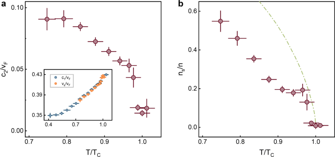
a Temperature dependence of the normalized first-sound speed c1/vF (blue dots in the inset) and second-sound speed c2/vF (red dots), obtained from the curve fitting of density response spectra Fig. 14. Here, \(v_{F}=\hbar k_{F}/m\) is the Fermi velocity. The inset also shows the adiabatic sound speed vS/vF (orange dots), calculated by using \(v_{S}=\sqrt {c_{1}^{2}+c_{2}^{2}-v^{2}}\). b Temperature dependence of the superfluid fraction ns/n, compared with that of superfluid helium (green dash-dotted line). Adapted from Ref. [33]
By applying the well-known relation v2=(Ts2ns)/(mCVnn) or by using Eq. (12), the superfluid fraction ns/n can be directly determined, as shown in Fig. 15b. In the vicinity of the phase transition, the superfluid fraction is close to that of superfluid helium, as found earlier at Innsbruck [23]. By decreasing temperature to 0.97Tc, the unitary Fermi superfluid rapidly acquires about 20% superfluid component. As temperature further decreases, however, the data start to significantly depart from the case of superfluid helium, in sharp contrast to the earlier observation at Innsbruck.
The key results of the USTC experiment—the first and second sound attenuation—are presented in Fig. 16, along with the extracted transport coefficients by using the relations κ≃[(D1+D2)mn−4ηn/(3nn)]CV and η=3nm(D1+D2−Ds)/4. The temperature dependence of D1 and D2 below Tc might be understood from the relations D1∼η/(nm) and D2∼ηns/(nmnn) valid at low temperature [33]. As temperature decreases, the saturated D1 is consistent with a nearly constant shear viscosity and the rapid increase of D2 is due to the loss of normal fluid component, i.e., ns/nn→∞ as T→0. Very close to the superfluid transition (i.e., at T>0.95 Tc), all the sound diffusivities show a sudden rise, with a variation \(\delta D\sim 0.3\hbar /m\).
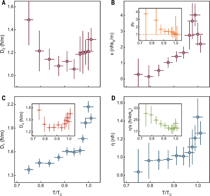
a The second-sound diffusivity D2. b The thermal conductivity κ. The inset shows the Prandtl number, with the line marking Pr=1. c The first-sound diffusivity D1, together with Ds in the inset. d The shear viscosity η. The inset reports the viscosity-to-entropy ratio, in units of \(\hbar /(4\pi k_{B})\). From Ref. [33]
In comparison with Fig. 2, it is remarkable that the second-sound diffusivity D2 of a unitary Fermi gas has a very similar temperature dependence as that of superfluid helium. The sudden rise in D2 near the superfluid transition then could be understood as a critical divergence, as we discussed earlier in superfluid helium section. Moreover, D2 clearly shows a minimum at T∼0.9Tc. Although the minimum value \((D_{2})_{\min }\simeq 1.1\hbar /m\) slightly smaller than the minimum D2 of superfluid helium given in Eq. (9), the important observation is that, there is a universal limit \(D\sim \hbar /m\) for both strongly interacting quantum fluids, due to the absence of well-defined quasi-particles.
Transport coefficients and quantum criticality
As in superfluid helium, the critical divergence in the second-sound diffusivity D2 near the superfluid transition should be attributed to the thermal conductivity κ, which diverges like |T−Tc|−ν/2≃|T−Tc|−1/3 both below and above Tc, according to the dynamic critical scaling theory of the superfluid transition [41, 42]. Indeed, as shown in Fig. 16b, there is a clear weak divergence on both sides of the superfluid transition, leading a pronounced peak around Tc with a significant height \(\delta \kappa \sim 3n\hbar k_{B}/m\). The Prandtl number Pr≡ηcP/κ is also reported in the inset. This number is about unity near the superfluid transition, suggesting that there the viscous damping and thermal damping are equally important to the sound attenuation. A similar Prandtl number has been found using Brillouin scattering in superfluid helium [45]. The near unity Prandtl number also implies that we may treat the unitary Fermi gas as a holographic conformal nonrelativistic fluid [67].
Finally, the shear viscosity is presented in Fig. 16d. It exhibits a weak temperature dependence below 0.95 Tc and becomes nearly constant, i.e., the quantum limit \(\eta \sim n\hbar \). In the vicinity of the superfluid transition, a smooth but significant increase is observed. The trap-averaged shear viscosity of a unitary Fermi gas in harmonic traps has been measured through anisotropic expansion [27], from which the locally uniform shear viscosity has also been indirectly extracted [28]. The shear viscosity in Fig. 16d turns out to be about two times larger than the previous data in the superfluid phase. Therefore, the unitary Fermi gas appears to be more viscous. As a quantitative measure, the viscosity-to-entropy ratio η/s is given in the inset, in units of the conjectured KSS low-bound \(\hbar /(4\pi k_{B})\) [66]. Around the transition, η/s is about 18 times larger than the bound, indicating that a unitary Fermi superfluid is a good but not the perfect fluid as we may anticipate.
Second sound in interacting Bose gases
First sound and second sound have also been measured in interacting Bose gases, both in two dimensions near the Berezinskii–Kosterlitz–Thouless (BKT) transition and in three dimensions, by Hadzibabic and his colleagues at University of Cambridge [34, 35]. Here, we briefly introduce their observations.
Second sound near the BKT transition
In the 2D experiment [34], a 2D homogeneous Bose gas of 39K atoms with surface density n≃3 μm−2 and area LxLy is prepared in a node of a vertical 1D optical lattice with a large harmonic trapping ωz=2π×5.5(1) kHz. Both the interaction and thermal energy per particle are below \(0.3\hbar \omega _{z}\), so the system is deep in the 2D regime. The s-wave scattering length is increased by a Feshbach resonance to a=522(23)a0 with the Bohr radius a0, so the dimensionless 2D interaction strength \(\tilde {g}=\sqrt {8\pi }a/\sqrt {\hbar (m\omega _{z})}=0.64(3)\) is large enough to maintain the collisional hydrodynamic behavior. There is a noticeable three-body loss due to the large interaction strength, but the system appears to decay slowly without heating and a steady-state may then be assumed.
At a given reduced temperature T/Tc, the Bose gas is perturbed by an in-plane, spatially uniformed force Fy(t)=F0 sin(ωt) created by a magnetic field gradient ΔB along the y-direction. The longest-wavelength sound mode(s) can then be excited, with wavenumber k=π/Ly. The resulting density fluctuation would assume the form, δn(y,t)/n=b(t) sin(ky), where the oscillating amplitude b(t) can be easily extracted from the displacement of the centre of mass of the cloud d(t)≡[R(ω) sin(ωt)−A(ω) cos(ωt)]∝b(t). The out-of-phase, absorptive response A(ω) then measures directly the imaginary part of the density response function Imχ(k,ω) at k=π/Ly.
In Fig. 17a, the normalized absorptive response \(\tilde {A}(\omega)\) is reported both below and above the BKT transition. The normalization is set according to the well-known f-sum rule [44, 52], \(\int \omega \tilde {A}(\omega)d\omega =c_{B}^{2}k^{2}\), with an appropriately chosen Bogoliubov sound velocity \(c_{B}=\sqrt {\tilde {g}n}\hbar /m\) and Bogoliubov frequency ωB=cBk as the units. The data have been fitted with two resonance functions, following the mode decoupling in Eqs. (35) and (36) (below Tc) or Eq. (37) (above Tc). Below the BKT transition at T=0.91Tc, two resonances with frequencies ω1>ω2 are clearly resolved, corresponding to the first sound and second sound, respectively. The sound velocities extracted from the resonance frequencies, i.e., c1=ω1/k and c2=ω2/k, are shown in Fig. 17b, as a function of the reduced temperature T/Tc. It is remarkable that the data can be well-explained by the theoretical results based on Landau’s two-fluid hydrodynamic theory [71–73], without any free parameters. These predictions have been obtained using the accurate equations of state and superfluid density from Monte Carlo simulations [74]. Moreover, at the BKT transition, a discontinuity in the second sound velocity can be clearly identified, due to the sudden jump of superfluid density.
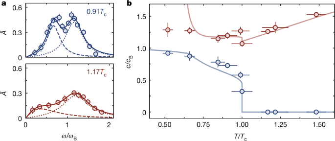
a Normalized density response spectra \(\tilde {A}(\omega)\) at 0.91Tc and 1.17Tc. Below Tc (top), two resonances corresponding to the first (dotted) and second (dashed) sound are observed. Above Tc (bottom), the first-sound resonance (dotted) exists, but the second sound is replaced by a diffusive, overdamped mode (dashed). b Normalized sound velocities, c1/cB (red) and c2/cB (blue), and the corresponding theoretical predictions for infinite-systems without any free parameters. The discontinuities in predicted velocities at Tc are due to the jump in superfluid density across the BKT transition. Adapted from Ref. [34]
The sound attenuations of both first sound and second sound can also be determined from the normalized absorptive response \(\tilde {A}(\omega)\), although they might be broadened by the loss-induced density drift. From the resonance widths, it has been found \(D_{1}=7(1)\hbar /m\) and \(10(2)\hbar /m\) for the first sound below and above Tc, respectively, and \(D_{2}=6(1)\hbar /m\) for the second sound below Tc. These sound diffusivities are several times larger than that of strongly interacting quantum fluids (i.e., superfluid helium or unitary Fermi gas).
Second sound in 3D compressible interacting Bose gases
The above measurements have been recently extended to a 3D interacting Bose gas confined in a cylindrical box trap of length L=70(2)μm in the z-direction and radius R=9.2(5)μm in the transverse direction [35]. The total number of atoms is N=105(3)×103 and the s-wave scattering length a=480(20)a0, leading to a gas parameter na3≃0.93×10⁻⁴. Although the relatively large gas parameter enhances the three-body loss and causes heating, the Bose cloud may still be treated as a quasi-equilibrium system at the time scale of about 100 ms. The reach of the hydrodynamic regime is characterized by klmfp∼0.47<1, where the wavenumber k=π/L for the lowest sound mode along the axis and lmfp=(8πna2)−1 is the collisional mean free path.
As in the 2D case, the lowest sound modes are excited by an axial magnetic gradient that imposes a spatially uniform force along the z-direction F(t)=F0 sin(ωt). After a variable time t, both the force and the trapping potential are turned off. The axial 1D momentum distribution nk(t) is then measured after a time-of-flight expansion of 30−45 ms. Consequently, the center-of-mass velocity \(v(t)=\hbar \left \langle k\right \rangle /m\) and current density j(t)=nv(t) are determined. This provides a complex optical conductivity σ(ω)∝j/F∝iωχ(k,ω) at k=π/L.
As shown in Fig. 18a, well below Tc (i.e., the top curve for T=0.77Tc), there are two well-resolved peaks in the spectrum |σ(ω)|2, which correspond to the first sound and second sound, respectively. The sound velocities cI and cII can be directly read from the peak positions ωI and ωII, i.e., cI,II=ωI,II/k. As reported in Fig. 18b, the temperature dependence of the two sound velocities can be well understood by applying a weak-coupling mean-field theory (see also Fig. 7a for a smaller gas parameter na3=10−5). The second sound attenuation may also be extracted. However, the deduced amplitude-damping coefficient does not show a clear dependence on the total number of atoms N.
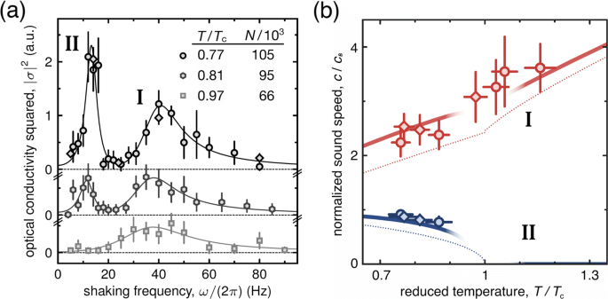
a Optical conductivity squared |σ(ω)|2 at three different reduced temperatures. The two peaks correspond to the two sound modes. The solid lines are fits using the sum of two resonances. b First (red) and second (blue) sound velocities, normalized by the Bogoliubov speed \(c_{B}=\sqrt {4\pi na}\hbar /m\), as a function of T/Tc. The solid lines are the fit-free predictions of the two-fluid model, with ns calculated using the Popov mean-field theory. The fade of the lines indicates the breakdown of the mean-field theory near Tc. The dotted lines show the sound velocities calculated by using non-interacting equation of state and condensate density (as superfluid density). Adapted from Ref. [35]
An interesting aspect of the 3D measurement is that the normal-fluid velocity vn(t) can be extracted from the high-momentum wing of the 1D momentum distribution nk(t). The superfluid velocity vs(t) can then be deduced from the total current j(t) based on the theoretical superfluid fraction. This provides an unique way to identify the microscopic structure of the second sound. As shown in Fig. 19a, at the second sound resonance, the extracted vn and vs are almost completely out-of-phase as the time evolves, as predicted for second sound.
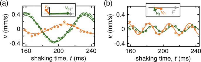
Microscopic structure of the two sound modes at T/Tc=0.77. a Extracted vn (orange) and vs (green) for the second-sound resonance, exhibiting the out-of-phase motion anticipated for second sound. b Analogous results for the first-sound resonance. Adapted from Ref. [35]
Conclusions and outlooks
In conclusions, the recent simultaneous observations of first sound and second sound propagations in strongly interacting unitary Fermi gases [23, 33] and in interacting Bose gases [34, 35] provide the textbook cases of the celebrated Landau’s two-fluid hydrodynamic theory [38, 39]. Unlike superfluid helium, both interacting Fermi gases and Bose gases are highly tunable and controllable systems [3], with the corresponding microscopic model Hamiltonians well established. Therefore, we now have an excellent toolbox to better understand the microscopic details of superfluidity and the superfluid phase transition in the strongly interacting regime.
In this respect, improved measurements of the unitary Fermi gas near the superfluid phase transition are of particular interest. In liquid helium, the investigations of critical divergences in the thermal conductivity κ above the λ-transition and in the second-sound diffusivity D2 below the λ-transition play a vital role in setting up the effective dynamic scaling theory for the critical mode across the superfluid transition [41, 42]. For a homogeneous unitary Fermi gas, the recent first measurement of both D2 and κ at USTC already indicates a much larger quantum critical regime, which is about 100 times larger than that of liquid helium. A systematic exploration of this large quantum critical region with improved temperature controllability could be achieved in the near future, paving the way to map out several long-sought universal critical dynamic scaling functions [42].
Future experiments on interacting Bose gases are equally important, as they present highly compressible examples of quantum liquids. However, the use of a large s-wave scattering length will cause three-body loss and heating, which prevent the precise determination of the sound velocities and sound attenuations. To overcome this difficulty, we may consider a molecular Bose–Einstein condensate, created by a two-component interacting Fermi gas on the BEC side. In particular, by adjusting the box-trap geometry and optimizing the system, the USTC setup in Fig. 13a can be readily modified to realize a two-dimensional homogeneous Fermi superfluid. This provides an ideal platform for investigating the first and second sound attenuation and related quantum transport across the BKT transition [75–77], without three-body loss.
Many-body challenges
The milestone experiments reviewed in this work already present a number of intriguing and challenging many-body problems for theorists. For example, both the superfluid density and the transport coefficients (shear viscosity η and thermal conductivity κ) of the unitary Fermi gas are notoriously to calculate theoretically. As shown in Fig. 20, the new data on the superfluid fraction from the USTC experiment lie between the theoretical predictions from the Gaussian pair fluctuation theory and the standard BCS mean-field theory. New calculations are definitively needed, to better explain the experimental observation (for a recent attempt, see Ref. [79]). In Fig. 21, the USTC results for the shear viscosity (blue circles) are compared with the local shear viscosity extracted from the trap-averaged shear viscosity [28] and the QMC calculations [78]. These results seem not to reach an agreement. Improved theoretical calculations of the shear viscosity of a unitary Fermi superfluid, based on either strong-coupling diagrammatic theories or QMC simulations, are timely required to resolve the discrepancy.
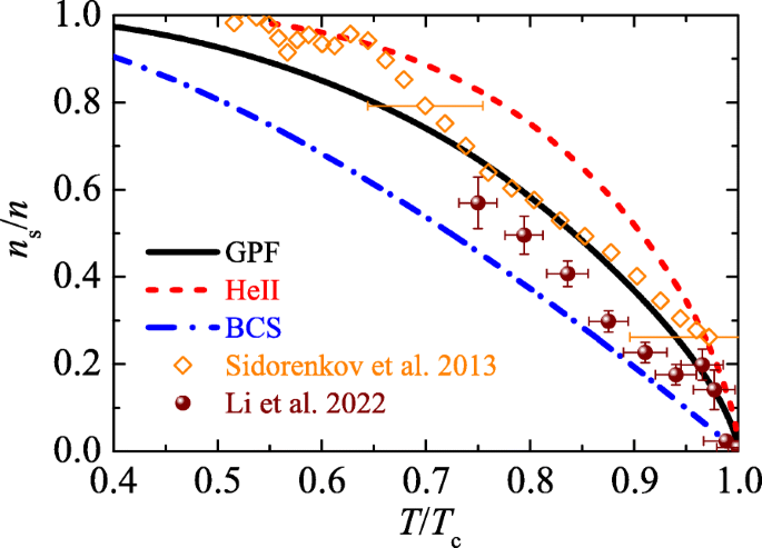
The superfluid fraction of a unitary Fermi gas measured from the Insbruck experiment in 2013 [23] (empty diamonds) and from the USTC experiment in 2022 (solid circles) [33], as a function of the reduced temperature T/Tc. The data are compared with the theoretical predictions from the Gaussian pair fluctuation (GPF) theory (black solid line) [14, 19] and mean-field BCS theory (blue dot-dashed line). The superfluid fraction of superfluid helium is also shown by a red dashed line
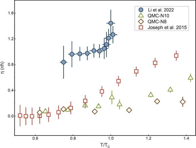
The shear viscosity of a unitary Fermi gas measured at NCSU in 2015 (empty squares) [28] and at USTC group in 2022 (solid circles) [33], as a function of the reduced temperature T/Tc. For comparison, we show also the quantum Monte Carlo simulations with lattice size N=83 (empty diamonds) and N=103 (empty triangles) [78]. From Ref. [33]
From the collisionless to hydrodynamic regime
On the other hand, less is known about the transition from the hydrodynamic regime to the collisionless regime. For unitary Fermi gas, the USTC setup can be easily extended to investigate the temperature and wave number dependence of the density response. As a result, the transition from collisionless to hydrodynamic behavior could be fully characterized and thus illuminate the establishment of hydrodynamics in the strongly interacting regime. We note that, in the normal state, the first sound density response at different wave numbers has been recently investigated by the NCSU group [80, 81]. The sound velocity and damping rate of zero sound in the collisionless regime have been studied by several experimental groups [82, 83] and have been theoretically addressed [84, 85].
For a compressible weakly interacting Bose gas, the collisionless to hydrodynamic transition in the normal state has been experimentally explored [35]. As reported in Fig. 22, the transition is tuned by the inverse Knudsen number L/lmfp for the lowest excitation mode with k=π/L. It is readily seen that, by increasing L/lmfp above 3 or decreasing klmfp down to 1, both the (first) sound velocity and its damping rate approach the predictions given by the full hydrodynamic calculations (solid lines). For such a three-dimensional weakly interacting Bose gas, it would be interesting to develop a quantitative microscopic description of the transition from the hydrodynamic regime to the collisionless regime [86]. In two dimensions close to the BKT transition, the sound propagation in an interacting Bose gas has also been experimentally observed by J. L. Ville et al. [87] and theoretically analyzed by using the random phase approximation [88] and the collisionless kinetic theory [89].
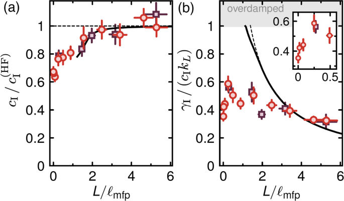
The first sound velocity (a) and its relative damping rate (b) of a 3D interacting Bose gas as a function of the inverse Knudsen number L/lmfp in its normal state at T≃1.3Tc. The first sound velocity is measured in units of cHF, given in Eq. (24). For large L/lmfp, the data approach the results of the full hydrodynamic calculation (solid lines). The inset in b highlights the damping in the collisionless limit. Adapted from Ref. [35]