Evolution of linear systems could be implemented with repeated action of linear operators. In finite-dimensional systems with randomness, the evolution may be computed with multiplication of random matrices. As a result, in diverse fields of science and engineering [1,2,3,4,5,6,7], random matrix products show up ubiquitously and have been a hot subject for intensive study for a long time [1]. In certain cases, the investigation is extended to the study of random products of operators as a generalization to infinite dimensions [8,9,10].

Among different aspects of random matrix products, the computation of the growth rate of their norms is of fundamental importance [1, 11, 12], which is related to the spectra of random oscillator chain [3, 13], the density of states in a disordered quantum system [4, 14,15,16,17] or the famous Anderson localization [18, 19]. However, few cases exist which can be solved with an exact analytic computation [11]. A common practice remains to be Monte carlo simulation which is easy to implement and thus used widely [1, 2, 20,21,22]. It is undoubtedly a good way to get a quick estimation of the growth rate. However, as well known, the convergence of the Monte carlo computation is slow, which in many cases prevents an accurate evaluation, especially when the growth rate is small. For good accuracy, sometimes cycle expansions could be used to extract the growth rate but its implementation quickly becomes rather involving if the number of the sampled matrices is large [23, 24]. To obtain analytic dependence on parameters, various perturbative techniques may be applied to get approximations such as the weak or strong disorder expansion [11, 25, 26]. Nevertheless, most of their application is focused on low-dimensional matrices and the computation sometimes turns out very technical even for low-order expansions [11].

In a recent paper [27], we proposed a generating function approach for the evaluation of growth rates of random Fibonacci sequences, which is very efficient and good for both analytic or numerical computation. Later on, the method is extended to random sequences with multi-step memory and a conjectured general structure in the generating function iteration is proved [28]. As the random sequence is a special case of random matrix products [1], it is thus tempting to see if this new formalism could be further extended. In the most general case, we succeeded in deriving such a new formulation along the previous line but with interesting new elements, which will be presented in this paper. Two methods of different sophistication for a perturbative expansion are proposed and demonstrated in a plethora of examples, where analytic expansions or even exact expressions in certain cases for growth rates are conveniently derived, for matrices with various dimensions or with different distributions.

The paper is organized as follows. In section 2, a general formulation of the random matrix product problem is proposed based on the generating function approach. In the next two sections, two different methods are suggested for the evaluation of growth rates based on the new formulation. The first one is a direct method which is easy to implement but somewhat restricted, to be discussed in section 3. The other one is an approach based on invariant polynomials which is more general but more involved, to be detailed in section 4. In these sections, both the analytic and the numerical computation is carried out and compared to check the validity of the new formulation. Then in section 5, the technique is applied to the calculation of the free energy of a random Ising model. Finally, problems and possible future directions are pointed out in section 6.

Here, after a brief review of the generating function technique in the evaluation of the grow rate of a random Fibonacci sequence, we reformulate the problem with 2×2 random matrices to give a taste of the new method. Then, a very general formulation is presented, which is good for random matrices of any dimension or with any probability distribution.

A brief review of the generating function approach to stochastic sequences

In a previous paper [27], we used a generating function approach to treat the generalized random Fibonacci sequence

In section 2.1, we see that the expansion in β is easily carried out to high orders just by several iterations of the recursion relation. This crisp feature could be maintained if the matrix A has a special structure. We will give several examples in the following to illustrate this point. To see the validity of the derived analytic expressions, Monte Carlo simulation is used for comparison. Each MLE is generated by carrying out one million Monte Carlo steps.

Expansion for 2-d matrices

To verify the validity of our procedure, we use the 2×2 matrices below

\(A=\left(\begin{array}{cc}a & b \\ c & d \end{array}\right) \pm \beta \left(\begin{array}{cc}e & r \\ g & h \end{array}\right).\)

(18)

In the above equation, if b=μa,d=μc, the argument substitution in Eq. (9) becomes x→μ±βR(x), where R(x) is a rational function of x. Thus, each additional iteration gives a higher order expression of λ in β when β is small.

More explicitly, if we take

\(A=\left(\begin{array}{cc} 3 & 0.3 \\ 2 & 0.2 \end{array}\right) \pm \beta \left(\begin{array}{cc}3 & 2 \\ 6 & 5 \end{array}\right),\)

(19)

where the plus or the minus sign is taken with equal probability, i.e. p(+)=p(−)=0.5, then a few iterations with Eq. (9) in view of Eq. (17) result in

\(\begin{aligned} \lambda(\beta)=&4\ln(2)-\ln(5)-\frac{156025}{131072}\beta^{2}+\frac{12034995625}{17179869184}\beta^{4} \\ &-\frac{2397118282953125}{844424930131968}\beta^{6}+O(\beta^{8}). \end{aligned}\)

(20)

In Fig. 1(a), the expansion Eq. (20) is compared with the results from the Monte carlo simulation. When β<0.3, the two agree very well while the error rises quickly after β=0.35. Especially, the valley at β∼0.42 is not present in the analytic result. This is because the expression Eq. (20) is an asymptotic one and is only valid for small β.

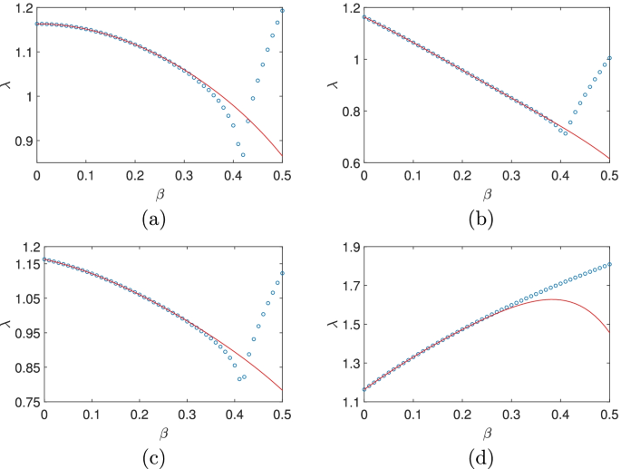
(Color online) The dependence of the MLE on β for different probabilities p of taking the plus and minus sign in Eq. (19). (a) p=0.5,0.5;(b) p=0.2,0.8;(c) p=0.4,0.6;(d) the result for the system with Eq. (24). The Monte carlo results are marked with (blue) circles while the analytic approximation is plotted with (red) solid line

 Full size image 

It is easy to see that in Eq. (20) there are only even powers of β since the plus or the minus sign is taken with equal probability and nothing changes if we change the sign of β. With different probabilities, e.g., p(+)=0.2,p(−)=0.8, we have

\(\begin{aligned} \lambda(\beta)=&4\ln(2)-\ln(5)-\frac{237}{256}\beta-\frac{100171}{131072}\beta^{2}+\frac{10169653}{8388608}\beta^{3}\\ &+\frac{8210001997}{17179869184}\beta^{4}+\frac{1202188020939}{5497558138880}\beta^{5}\\ &-\frac{5433460372890823}{1055531162664960}\beta^{6}+O(\beta^{7}), \end{aligned}\)

(21)

which is plotted in Fig. 1(b) and matches well with the simulation result. Here, in the expression Eq. (21), both even and odd powers of β are present as expected. To further see the trend, we take p(+)=0.4,p(−)=0.6 which gives

\(\begin{aligned} \lambda(\beta)=&4\ln(2)-\ln(5)-\frac{79}{256}\beta-\frac{149819}{131072}\beta^{2}+\frac{11994217}{25165824}\beta^{3}+\frac{11371586637}{17179869184}\beta^{4} \\ &+\frac{4828258136419}{16492674416640}\beta^{5}-\frac{10112843356609571}{3166593487994880}\beta^{6}+O(\beta^{7}), \end{aligned}\)

(22)

being plotted in Fig. 1(c). From the above three plots and more plots not shown, we see that one singularity emerges near β∼0.42, almost independent of the probability distribution. Also, the analytic result agrees with that of the simulation in a region of decreasing size as p(+) increases which is probably related to the positiveness of all the elements in the two matrices in Eq. (19). Also, as p(+) approaches 0.5, the absolute values of the coefficients of the odd powers of β become smaller and smaller and vanish at β=0.5 while those of the even powers rise considerably.

To check the validity of the method in more complicated cases, we consider the following situation

\(A=\left(\begin{array}{cc} 3 & 0.3 \\ 2 & 0.2 \end{array}\right) + \beta B_{i},i=1,2,3,\)

(23)

where

\(B_{1}=\left(\begin{array}{cc}3 & 2 \\ 6 & 5 \end{array}\right), B_{2}=\left(\begin{array}{cc}4 & 2 \\ 1 & 5 \end{array}\right), B_{3}=\left(\begin{array}{cc}3 & 5 \\ 1 & 2 \end{array}\right),\)

(24)

and p(1)=1/6,p(2)=1/6,p(3)=2/3. Our iteration gives

\(\begin{aligned} \lambda(\beta)=&4\ln(2)-\ln(5)+\frac{1865}{1024}\beta-\frac{47835425}{28311552}\beta^{2}\\ &+\frac{16396501375}{7247757312}\beta^{3}-\frac{198183253204375}{44530220924928}\beta^{4}\\ &+\frac{208937303364213625}{17099304835172352}\beta^{5}\\ &-\frac{1976335641588741029125}{52529986053649465344}\beta^{6}+O(\beta^{7}), \end{aligned}\)

(25)

which is plotted and compared favourably with the numerical result in Fig. 1(d). In all the examples above, the absolute values of the coefficients approximately increase exponentially with the powers of β which indicates a finite radius of convergence of the asymptotic expansion.

Expansion for 3-d and 4-d matrices

Our scheme is independent of the dimension of the involved matrices. Below, we show the computation on the 3×3 or 4×4 matrices. Here, we give one example for each case.

If we take the 3d matrices to be

\(A=\left(\begin{array}{ccc} 3 & 0.3 & 0.3\\ 2 & 0.2 & 0.2\\ 4 & 0.4 & 0.4 \end{array}\right) \pm \beta \left(\begin{array}{ccc}5 & 2 & 1\\ 2 & 1 & 3\\ 3 & 1 & 4 \end{array}\right)\)

(26)

with p(+)=p(−)=0.5, then the MLE is

\(\begin{aligned} \lambda(\beta)=&\ln(2)+2\ln(3)-\ln(5)-\frac{1965145}{839808}\beta^{2}-\frac{3740078636935}{705277476864}\beta^{4} \\ &-\frac{2664607365123862205}{22211625233825792}\beta^{6}+O(\beta^{8}). \end{aligned}\)

(27)

As before, the symmetry in the plus and minus sign results in the presence of only even powers of β. As shown in Fig. 2(a), the analytic result Eq. (27) matches well with the numerical result when β<0.38. If we take p(+)=0.4,p(−)=0.6, then

\(\begin{aligned} \lambda(\beta)=&\ln(2)+2\ln(3)-\ln(5)-\frac{277}{648}\beta-\frac{363133}{155520}\beta^{2}\\ &-\frac{1155711217}{2040733440}\beta^{3} -\frac{460024252888567}{88159684608000}\beta^{4}\\ &-\frac{903051494441389}{2380311484416000}\beta^{5} \\ &-\frac{56063372931443174652157}{4916533371061248000000}\beta^{6}+O(\beta^{7}), \end{aligned}\)

(28)

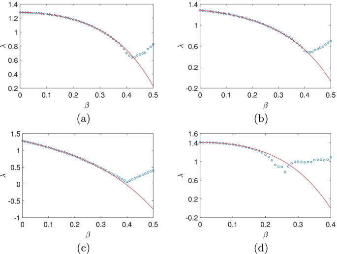
(Color online) The dependence of the MLE on β. For Eq. (26) with (a) p(+)=p(−)=0.5; (b) p(+)=0.4,p(−)=0.6; (c) p(+)=0.1,p(−)=0.9; (d) For the system given by Eq. (30) with p(+)=p(−)=0.5. The Monte carlo results are marked with (blue) circles while the analytic approximation is plotted with (red) solid line

 Full size image 

which is plotted in Fig. 2(b). If we take p(+)=0.1,p(−)=0.9, then

\(\begin{aligned} \lambda(\beta)=&\ln(2)+2\ln(3)-\ln(5)-\frac{277}{162}\beta-\frac{3162527}{1399680}\beta^{2}-\frac{2280847319}{1020366720}\beta^{3}\\ &-\frac{349001178994027}{88159684608000}\beta^{4}-\frac{10734200281829}{6198727824000}\beta^{5}\\ &-\frac{47383578974881029764663}{1966613348424499200000}\beta^{6}+O(\beta^{7}), \end{aligned}\)

(29)

which is plotted in Fig. 2(c). From Eqs. (27),(28) and (29), we see that the absolute values of the coefficients of the odd powers in the expansion increase with the decrease of p(+), while the validity domain of the expansion increases. The location of the singularity is more or less stable in the figure where the simulation result bends off the analytic approximation.

In the 4d case, we take

\(A=\left(\begin{array}{cccc} 3 & 0.3 & 0.3 & 0.3\\ 2 & 0.2 & 0.2 & 0.2\\ 4 & 0.4 & 0.4 & 0.4 \\ 5 & 0.5 & 0.5 & 0.5 \end{array}\right) \pm \beta \left(\begin{array}{cccc}5 & 2 & 1 & 3\\ 2 & 1 & 3 & 4\\ 3 & 1 & 1 & 5\\ 1 & 3 & 2 & 4 \end{array}\right)\)

(30)

with p(+)=p(−)=0.5. The MLE is then

\(\begin{aligned} \lambda(\beta)=&\ln(41)-\ln(2)-\ln(5)-\frac{11900886}{2825761}\beta^{2} \\ &-\frac{228277459672908}{7984925229121}\beta^{4}+O(\beta^{6}), \end{aligned}\)

(31)

which is plotted in Fig. 2(d) together with the numerical result. From the figure, we see that the validity region of Eq. (31) reduces again compared to the 2d or 3d cases. Also, the dependence on β becomes quite complex after β∼0.2.

In all the above computations, in order to carry out the computation, the β−independent part of the matrix has a very special form, which may be considered as a limitation of the method. However, in practice, for a fixed β, we are always allowed to freely choose that part of the matrix by properly adjusting the random parts. The real problem is how to choose a good one to make a quick convergence of the expansion. An empirical hint is to make the stochastic part as small as possible.

Direct expansion for continuous distribution

We use one example to demonstrate the application of the current technique to matrices with continuous distribution. With the specific matrices and distribution below, we are able to derive an exact analytic expression of λ, which could be used to explain the failure of the asymptotic expansion.

We use the following 2×2 matrices

\(A=\left(\begin{array}{cc} 1 & 1 \\ 1 & 1 \end{array}\right) + \beta \left(\begin{array}{cc}0 & -2 \\ 0 & -2 \end{array}\right),\)

(32)

and the distribution of β is assumed to be uniform in the interval [0,α] with

\(p(\beta)=\frac{1}{\alpha},\)

(33)

for a given α>0. The substitution Eq. (14) becomes

\(\tilde{z}_{2}=1-2\beta.\)

(34)

In this particular case, after one iteration, the variable z₂ in the expression f_n disappears and thus f_n becomes a constant. In other words, an exact expression of λ is obtained as

\(\lambda(\alpha)=\frac{(\alpha-1)\ln(1-\alpha)+\alpha(\ln(2)-1)}{\alpha},\)

(35)

and its direct expansion around α=0 is

\(\begin{aligned} \lambda(\alpha)=&\ln(2)-\frac{1}{2}\alpha-\frac{1}{6}\alpha^{2}-\frac{1}{12}\alpha^{3}-\frac{1}{20}\alpha^{4}\\ &-\frac{1}{30}\alpha^{5}-\frac{1}{42}\alpha^{6}+O(\alpha^{7}). \end{aligned}\)

(36)

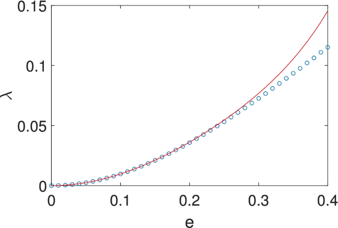
The above two solutions are plotted in Fig. 3 and compared with the results from the Monte Carlo simulation. It is easy to see that the exact result matches well with the Monte carlo simulation for all α. Nevertheless, the asymptotic expansion starts to deviate near α∼1, due to the truncation of high order terms. So, the singularity at α=1 in the logrithmic function plays a central role in the convergence of the asymptotic series here. Even though the convergence is very good for small α, near the singularity the expansion could totally go awry, which may also explain the sudden explosion of the error in the asymptotic expansion in Figs. 1 and 2.

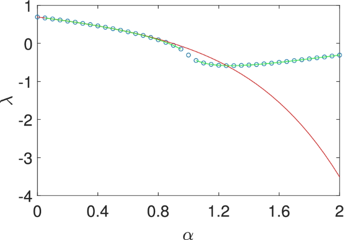
(Color online) The dependence of the MLE on α for the system described by Eq. (32). The Monte carlo result is marked with (blue) circles while the exact one is plotted with (green) solid lines. The analytic approximation is plotted with (red) solid lines

 Full size image 

Below, the major deterministic part of the random matrix A is denoted as A₀, which is the matrix for β=0. As explained before, although the direct expansion technique is fast and convenient, it could be a problem to extract a proper matrix A₀ with the required special structure. In this section, a more sophisticated expansion based on invariant polynomials is introduced to cope with this difficulty.

A general formulation

In the study below, the matrix A₀ is always considered to be diagonalizable. For simplicity, we assume that this has already been done and

\(A=\text{Diag}(\lambda_{1},\lambda_{2},\cdots,\lambda_{k+1}) \text{ with} \lvert\lambda_{1}\rvert>\lvert\lambda_{2}\rvert>\cdots>\lvert\lambda_{k+1}\rvert,\)

where λ_i’s are eigenvalues of A. With this simplification, the substitution in Eq. (13) is greatly simplified. Especially, the deterministic part of \(\tilde {z}_{i}\) (see Eq. (14)) becomes λ_iz_i/λ₁,i=2,3,⋯,k+1. If we assume that all z_i’s are small, all \(\tilde {z}_{i}\)’s could essentially be approximated by polynomials of {z_i}_i=2,⋯,k+1 up to a given order m. In fact we can do a Taylor expansion of the denominator of Eq. (14) to the order m to get these polynomials. The starting Eq. (16) could also be expanded to the same order, i.e., we may start with an m-th order polynomial

\(f_{0}(𝔃)=\sum\limits_{i=0}^{m} a_{i} 𝔃^{i},\)

(37)

where the short-hand notation i is a collective index for {i₂,⋯,i_k+1} and

\(𝔃^{i}=\Pi_{j=2}^{k+1}z_{j}^{i_{j}},\text{ with} \sum\limits_{j=2}^{k+1} i_{j}=i.\)

(38)

With the polynomial substitution and the ensuing truncation to the m-th order, the polynomial f_n(z) will approach a stationary form which is invariant under the iteration, since |λ_i/λ₁|<1 and the random term B(α) is assumed small.

Alternatively, we may assume that the polynomial f₀(z) in Eq. (37) is already invariant and seek for appropriate coefficients a_i. Upon one iteration, these coefficients become \(\tilde {a}_{i}\) that are linearly related to the original coefficients, i.e.

\(\tilde{a}_{i}=C_{ij} a_{j},\)

(39)

where C is the transformation matrix that depends on the random matrices B(α) and their sampling rates. The invariance condition predicts that C has 1 as its dominant eigenvalue and the absolute values of all other eigenvalues are smaller than 1. The corresponding left eigenvector L and right eigenvector R could be obtained by solving the linear equation

\((C_{ij}-\delta_{ij})R_{j}=0,\text{ and} (C_{ij}-\delta_{ij})L_{i}=0,\)

(40)

where δ_ij is the Kronecker delta function.

The starting function Eq. (16) could of course be expanded into a polynomial form with the coefficient vector b_i, which could be written as a linear combination of right eigenvectors. Upon iterations, with the assumed spectral property of matrix C, the first mode remains intact and all the other ones decays to zero. As a result, the final stationary coefficient vector \(\bar {b}_{i}\) is the projection of the starting vector b_i to the first eigenvector which can be computed as

\(\bar{b}_{i}=\frac{\sum_{j} L_{j} b_{j}}{\sum_{j} L_{j} R_{j}}R_{i}.\)

(41)

From Eq. (17), the constant term \(\bar {b}_{0}\) in the invariant polynomial gives the MLE. In fact, it is not hard to see that the right eigenvector could be taken as R_i=δ_i0, corresponding to a zeroth order polynomial, which is obviously invariant under the iteration. Therefore,

\(\lambda=\frac{\sum_{j} L_{j} b_{j}}{L_{0}},\)

(42)

which will be checked in several examples below.

Two examples

Here, we give two examples for the application of the method of invariant polynomials. For simplicity, we assume that when β=0, the major part of the matrix is already in a diagonal form. In the two dimensional case, we take

\(A_{n}=\left(\begin{array}{cc}3 & 0 \\ 0 & 2 \end{array}\right) \pm \beta \left(\begin{array}{cc}2 & 0.5 \\ 1.2 & 3.0 \end{array}\right)\)

(43)

with p(+)=p(−)=0.5. A direct application of the above scheme gives the growth rate

\(\lambda(\beta)=\ln(3)-\frac{2}{9}\beta^{2}+\frac{719}{20250}\beta^{4}-\frac{774479}{13668750}\beta^{6}+O(\beta^{8}),\)

(44)

where only even powers of β are present due to the sign symmetry mentioned previously. A comparison of the computation from Eq. (44) and from numerical computation is displayed in Fig. 4(a). It is easy to see that the two results agree very well in the whole computational region. In the case of 3×3 matrices, we try

\(A=\left(\begin{array}{ccc} 4 & 0 & 0\\ 0 & 2 & 0\\ 0 & 0 & 3 \end{array}\right) \pm \beta \left(\begin{array}{ccc}2 & 1.2 & 0.6\\ 0.5 & 0.7 & 2\\ 3 & 1 & 0.4 \end{array}\right)\)

(45)

(Color online) Comparison of the expansion result with the numerical computation for the systems givey by (a) Eq. (43), (b)Eq. (45). The Monte carlo results are marked with (blue) circles while the analytic approximation is plotted with (red) solid lines

 Full size image 

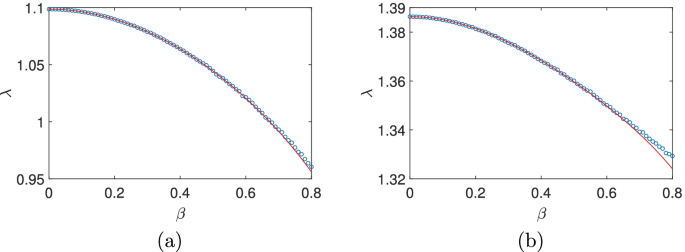
with p(+)=p(−)=0.5. The maximum Lyapunov exponent is

\(\begin{aligned} \lambda(\beta)=&2\ln(2)-\frac{1}{8}\beta^{2}+\frac{926378511}{13421772800}\beta^{4}\\ &-\frac{1771471938223}{64424509440000}\beta^{6}+O(\beta^{8}), \end{aligned}\)

(46)

which is plotted in Fig. 4(b) together with the numerical profile. The two agree quite well until β∼0.7, which nicely confirms the validity of our new scheme based on invariant polynomials.

In this section, we apply our method to the one-dimension Ising model with random on-site field. In this model, N spins lay side by side along a one-dimensional lattice, each of which has two possible states: the spin up state (σ_i=1), or the down state (σ_i=−1). Following the terminology in [1], we may write down the Hamiltonian of the system

\(H=-J\sum\limits_{i=1}^{N}\sigma_{i}\sigma_{i+1}-\sum\limits_{i=1}^{N} h_{i}\sigma_{i},\)

(47)

where J is the coupling constant between nearest-neighbor spins and h_i is the external magnetic field on each site, being assumed to be random. The first term in Eq. (47) describes the interaction of neighboring spins and the second term takes into account the potential energy in the external field. The partition function is

\(Z_{N}=\sum\limits_{\{\sigma\}} \exp(\beta J \sum\limits_{i} \sigma_{i} \sigma_{i+1}+ \beta \sum\limits_{i} h_{i} \sigma_{i}).\)

(48)

Introducing the transfer matrix

\(L_{i}(\sigma_{i},\sigma_{i+1})=\exp(\beta J \sigma_{i} \sigma_{i+1}+\beta h_{i}\sigma_{i}),\)

(49)

or more explicitly

\(\begin{aligned} L_{i}=\left(\begin{array}{cc} L_{i}(1,1) & L_{i}(1,-1) \\ L_{i}(-1,1) & L_{i}(-1,-1) \end{array}\right) =\left(\begin{array}{cc} e^{\beta(J+h_{i})} & e^{\beta(-J+h_{i})} \\ e^{\beta(-J-h_{i})} & e^{\beta(J-h_{i})} \end{array}\right), \end{aligned}\)

(50)

with a periodic boundary condition, the free energy per spin could be written as

\(F=-{\underset{N\to\infty}{\lim}}\frac{1}{\beta N}\ln Z_{N}=-{\underset{N\to\infty}{\lim}}\frac{1}{\beta N}\ln[Tr(\prod\limits_{i=1}^{N}L_{i})].\)

(51)

The equations above provide a general frame of computing the free energy of the 1-d Ising model using the transfer matrix approach. An exact analytic expression may be derived if the external field is constant over the sites. In the presence of local randomness, the external field h_i is a quenched random variable, differing from site to site, for which it is hard to get an exact solution. When the interaction is strong, an analytic expansion is easily derived with our method. First, we reshape Eq. (50) as follows

\(\begin{aligned} L_{i}=e^{\beta(J+h_{i})}\left(\begin{array}{cc} 1 & e^{-2\beta J} \\ e^{-2\beta(J+h_{i})} & e^{-2\beta h_{i}} \end{array}\right) =e^{\beta(J+h_{i})} \left(\begin{array}{cc} 1 & \epsilon \\ \epsilon x_{i} & x_{i} \end{array}\right) \end{aligned}\)

(52)

with \(x_{i}=e^{-2\beta h_{i}}\) and ε=e^−2βJ, being small and to be used as the expansion parameter. When the reshaped L_i is used in Eq. (51), the free energy could be written as [1]

\(F=-J-\overline{h}-\frac{1}{\beta}{\underset{N\to\infty}{\lim}}\frac{1}{N}\ln[Tr(\prod_{i=1}^{N}\left(\begin{array}{cc} 1 & \epsilon \\ \epsilon x_{i} & x_{i} \end{array}\right))]\)

(53)

\(\overline {h}\) is the average of h_i over different sites. Once the distribution of ε is given, the first and the second term in Eq. (53) are obtained directly. What is left to do is a proper estimation of the third term. Since the major part of the third term is diagonal, we may directly apply our method to compute

\(\lambda={\underset{N\to\infty}{\lim}}\frac{1}{N}\ln[Tr(\prod_{i=1}^{N}\left(\begin{array}{cc} 1 & \epsilon \\ \epsilon x_{i} & x_{i} \end{array}\right))].\)

(54)

For simplicity, we assume a uniform distribution of x_i in (0,1), i.e. P(x)=1. Other forms of distributions can equally be used in our formulation while the resulting quadrature may not be computed analytically. The variable substitution Eq. (14) looks simple now

\(\tilde{z}_{2}=\frac{\epsilon+x z_{2}}{1+\epsilon x z_{2}},\)

(55)

and the starting function has a integral form

\(f_{0}(z_{2})=\int_{0}^{1}P(x)\ln(1+\epsilon x z_{2})dx,\)

(56)

since the distribution is continuous. The method of invariant polynomials may be applied here by expanding Eq. (55) and (56) into polynomials of proper order depending on the desired accuracy. For example, if the expansion is carried out to the sixth order, we may obtain

\(\lambda(\epsilon)=\epsilon^{2}-\frac{269}{90}\epsilon^{4}+\frac{392309}{25920}\epsilon^{6}+O(\epsilon^{8}),\)

(57)

the leading order of which agrees with that in [1] for this particular distribution. In Fig. 5, we see that the analytic result matches well with the numerical one when ε<0.3. The free energy of the system reads

(Color online) A comparison of the analytic approximation with the numerical simulation for Eq. (57). The Monte carlo results are marked with (blue) circles while the analytic approximation is plotted with (red) solid line

 Full size image 

\(\begin{aligned} F=&-\frac{1}{2}-J-\frac{e^{-4 \beta J}}{\beta}-\frac{269e^{-8 \beta J}}{90 \beta}\\ &+\frac{392309e^{-12 \beta J}}{25920 \beta}+O(e^{-16 \beta J}). \end{aligned}\)

(58)

The Taylor expansion is valid only when ε is small so that Eq. (58) is a good approximation for J large enough.

In this paper, we generalize the generating function approach developed in [27, 28] for dealing with stochastic sequences to the treatment of random matrix products. After a general formalism is introduced, two analytic schemes are designed for the computation of the MLE: a direct iteration scheme and a more sophisticated one based on invariant polynomials. Several examples are given to illustrate the usage of the methods. As expected, when the randomness is small (β small), the analytical results agree very well with the numerical ones. However, with the increase of randomness, the agreement becomes worse and higher order terms may chip in playing a role. In many cases, the increase of randomness brings in complex dependence of the MLE on β which can not be captured by an analytic expansion [2, 21]. When the current technique is used in the study of an Ising model with random onsite fields, the free energy is conveniently obtained with an analytic approximation in case of a strong coupling between neighboring spins.

The direct iteration scheme is very easy to implement but requires a special form of the major part of the random matrix which may not be determined so straightforwardly in practice. The second scheme based on invariant polynomials is very general but requires solution of a linear equation. Also, we assume that the major part of the random matrix has one dominant eigenvalue to guarantee a good convergence of the expansion. If there are multiple eigenvalues that have the same magnitude, the convergence of the polynomial coefficients is not guaranteed and we have to modify the method. On the other hand, as implemented in [27, 28], with the generating function formalism, a numerical scheme could be easily designed for the computation of the growth rate for any value of β, which is at least good for small matrices. For large matrices, however, a direct numerical computation seems unmanageable. Whether it is possible to extend either of the current two schemes to highly efficient numerical tools is an interesting question.

In the examples given above, matrices with dimensions only up to 4 are used in the computation although the formulation is valid for random matrices of higher dimensions. Of course, even the analytic computation could become cumbersome in high-dimensional cases, especially for the method based on invariant polynomials, if the involved random matrices are present in a large quantity. Nevertheless, even for a continuous distribution of matrices, the current scheme applies well [27], as demonstrated in the example in Section 3.3, as long as the involved integration is not hard to do.

In all the above computation, only the MLE is computed. How to generalize the current formulation to the evaluation of other Lyapunov exponents is still under investigation. Also, in all the calculations, we assume that the MLE exists which measures the exponential increase of the length of a typical vector following the dynamics determined by random matrix multiplication. However, in certain critical cases, this growth may not be exponential but follows a power law [21]. How to adjust the above computation to this case is still an open problem [29,30,31,32].