The formal valences of elements have been empirically compiled through the systematic chemical studies of many compounds. Figure 1 shows a periodic table indicating the valences of elements determined through analysis of various compounds [1]. Some elements have a single valence, while others have several different valences. For example, oxygen (O) in compounds exists only as an anion with a charge of − 2, while sulfur (S) can have not only an anionic charge of − 2, but also the cationic charges of + 4 and + 6.

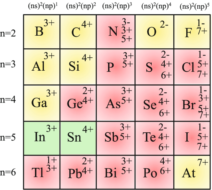
Periodic table indicating the valences of elements determined through analyses of a series of compounds [1]. Elements indicating by a red gradation are valence skippers. It should be noted that the valence state of Sn ion and In ion is 4+ for Sn ion and 3+ for In ion in Ref. [1]. However, because the valence skipping phenomenon of these elements have been studied recently as discussed in Sec. 5, we show these elements by the green gradation

 Full size image 

The valences assumed by anions are clearly related to the closed shell structure of atoms. For example, the anion state of nitrogen (N) and (O) correspond to the closed shell structure, because the electronic states of N ³⁻ and O ²⁻ ions are 1s²2s²2p⁶3s²3p⁶ and 1s²2s²2p⁶ states, respectively. On the other hand, in the cation cases, when we focus on the valence state of S, these valence states of S ⁴⁺ and S ⁶⁺ are 1s²2s²2p ⁶3s² and 1s²2s²2p⁶, respectively: the 3s orbital of S ⁶⁺ state is a closed shell structure, and 3s orbital is doubly occupied by spin-up and spin-down electrons in S ⁴⁺ state. As in the case of S, the elements located in group V takes the special ionic states. For example, Tl ion takes valences Tl ¹⁺ (6s²) and Tl ³⁺ (6s⁰) but not Tl² (6s¹), and Bi ion takes valences Bi ³⁺ (6s²) and Bi ⁵⁺ (6s⁰) but not Bi ⁴⁺ (6s¹). As discussed above, the formal ionic states of many elements have a tendency to take the closed shell structure of ns⁰ and ns² states. In other words, ns¹ state has a tendency to be skipped. This phenomenon has been known as valence skipping, and the element indicating the valence skipping is called as valence skipper. In the field of chemistry, in terms of the stability of ns² state, this phenomenon is named as inert pair effect or lone pair effect.

Historically, the valence skipping has been deeply discussed in terms of the relationship with a negative-U effect, which introduces in Section 2.1, while the superconductivity emerging from the valence skipping have been studied extensively since 1990s, starting with the suggestion of the superconductivity due to the new mechanism deriving from the valence skipping phenomena of Bi ion in (Ba,K)BiO₃ (BKBO) [2]. After BKBO, by the discovery of the charge Kondo effect and superconductivity in Tl-doped PbTe [3], the valence skipping have been focused again. In addition, recently, the microscopic theory of the valence skipping phenomena due to the pair hopping interaction has been suggested [4], and experimentally, the dynamical features of the valence skipping phenomena has been revealed by the nuclear magnetic resonance (NMR) [5]. Then, there are many candidate materials, expecting a valence skipping induced superconductivity as shown in Section 5. Therefore, in this paper, we review a theoretical and experimental progress concerning the superconductivity and the charge Kondo effect induced by the valence skipping.

The organization of the paper is as follows. In Section 2, we recapitulate the relationship between valence skipping state and a negative-U effect, and we briefly survey the theories for negative-U effects reported so far. In Section 2.2, we review the theory for superconductivity of BKBO on the idea of negative-U effect. In Section 3, we present a new microscopic theory for the valence skipping phenomena and the charge Kondo effect on the basis of the pair-hopping interaction, and we sketch a possible superconducting mechanism in a two-band lattice system on the basis of the pair-hopping interaction which is the heart of the charge Kondo effect and valence-skipping phenomenon. In Section 4.1, we introduce the experiments in Tl-doped PbTe which exhibits superconductivity and Kondo-like behavior in the resistivity, and some macroscopic experiments, and explain the theoretical analysis based on the negative-U model in Section 4.2. In Section 4.3 and Section 4.4, the anomaly of NMR relaxation rate 1/T₁ are discussed both from experimental and theoretical aspects. Finally, in Section 5, the candidate materials expected in the future are introduced.

Negative-U model

As discussed in the introduction, the valence skipping phenomenon is related to the stability of a pair of electrons in the ns orbital. To understand this stability qualitatively, we consider the energetics on a simple Hamiltonian as

\(\begin{array}{@{}rcl@{}} H = U_{\mathrm{s}}n_{\uparrow}n_{\downarrow} +\epsilon_{\mathrm{s}}(n_{\uparrow} + n_{\downarrow}), \end{array}\)

(1)

where U_s and ε_s are the effective Coulomb interaction between electrons on ns orbital, and one-body level of ns electron, respectively. n_σ is a number of electron with spin σ on ns orbital. Then, the total energy, E_m, where m (m=0,1,2) is the number of electrons on ns orbitals, is given as

\(\begin{array}{*{20}l} E_{0} = 0, \end{array}\)

(2)

\(\begin{array}{*{20}l} E_{1} = \epsilon_{\mathrm{s}}, \end{array}\)

(3)

\(\begin{array}{*{20}l} E_{2} = 2\epsilon_{\mathrm{s}} +U_{\mathrm{s}}. \end{array}\)

(4)

As discussed above, the condition for the valence skipping state to be realized is that ns¹ state has the energy higher than that of ns⁰ or ns² state. Namely, the condition is given by

\((E_{2} +E_{0})/2 < E_{1}.\)

(5)

Figure 2 shows a schematic picture of the condition. The inequality Eq. (5) implies that the effective Coulomb interaction U_s between ns electrons is negative, the situation of which is regarded to be caused by the “negative-U effect”.

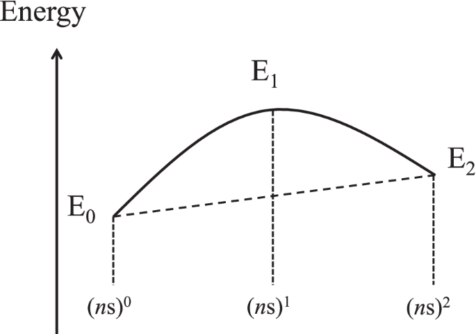
Schematic picture of energy levels

 Full size image 

Origin of negative-U effect

In Section 2.1, we have used the phenomenological model with the negative-U interaction. Here, we briefly review ideas for the origin of the negative-U interaction.

The orgin of negative-U based on the electron-lattice interaction was first proposed by Anderson [6]. The potential energy of the ith atom (ion) is

\(\begin{array}{@{}rcl@{}} V =\frac{1}{2}cx_{i}^{2} -\lambda x_{i} (n_{i\uparrow}+ n_{i\downarrow}), \end{array}\)

(6)

where x_i is the distance from the center of ith site, c is a constant, λ is the coupling constant of electron-lattice interaction, and n_i↑ and n_i↓ are number of electrons with up and down spins at ith site, respectively. By minimizing V(x_i) with respect to x_i, the minimum of the potential energy, V_min, is given by V_min=−λ²/c. Therefore, the effective Coulomb interaction at ith site is given by

\(\begin{array}{@{}rcl@{}} U_{\text{eff}} = U -\frac{\lambda^{2}}{c} \end{array},\)

(7)

where U is the screened Coulomb interaction between electrons at ith site. In the case U<λ²/c,U_eff<0 leading to a negative-U effect. Recently, the relation between the electron-lattice interaction and charge Kondo effect has been discussed by the numerical renormalization group calculations on the basis of Anderson-Holstein model, which includes the electron-lattice interaction [7, 8].

The another possibility of negative-U effect has been discussed by Varma [2] through estimating the total energy of ionic state on each elements. The effective Coulomb interaction U_n between electrons on ions with the valence state n+ is defined as

\(\begin{array}{@{}rcl@{}} U_{n} \equiv (E_{n+1} -E_{n}) + (E_{n-1} - E_{n}), \end{array}\)

(8)

where E_n is the total energy of n+ ionic state. Table 1 shows the values of U_n for elements in group 13, 14, and 15 in periodic table. This results show that U_n is positive and is not negative, while U_n at the valence number of valence skipping tends to have smaller value. However, this discussion is based on the isolated atoms (ions). In the real system such as (Ba _1−xK_x)BiO₃, there are oxygens around cation, such as Bi ion. Therefore, it was suggested that the screening effect, due to the transition of electrons from the oxygen, is important for the reduction of U_n [2].

Table 1 The effective Coulomb interaction in ions

Group 13	U 1+(s2)	U 2+(s1)	U 3+(s0)
Ga	14.6	9.2	26.4
In	13.1	9.2	26.4
Tl	14.3	9.4	20.9
Group 14	U 2+	U 3+	U 4+
Ge	18.2	9.5	48.7
Sn	15.9	9.1	31.6
Pb	16.9	10.4	25.5
Group 15	U 3+	U 4+	U 5+
Sb	18.8	11.9	52.0
Bi	19.7	10.7	32.3

Hase and Yanagisawa calculated the Madelung energy in the case of the charge ordered state of Bi ³⁺ and Bi ⁵⁺, and Bi ⁴⁺ in the case of BaBiO₃, and discussed the condition for U_n to become negative [9]. The energy difference between the charge ordered state of Bi ³⁺ and Bi ⁵⁺, and the normal state of only Bi ⁴⁺ ions is

\(\begin{array}{@{}rcl@{}} & &\Delta E = \left[E\left(\text{Ba}_{2}^{2+}\text{Bi}^{3+}\text{Bi}^{5+}\mathrm{O}_{6}^{2-}\right) +E_{\text{ion}}\left(\text{Bi}^{5+}\right)+ E_{\text{ion}}\left(\text{Bi}^{3+}\right)\right] \\ & &\qquad\quad - \left[E\left(\text{Ba}_{2}^{2+}\text{Bi}^{4+}\text{Bi}^{4+}\mathrm{O}_{6}^{2-}\right) +2E_{\text{ion}}\left(\text{Bi}^{4+}\right)\right], \end{array}\)

(9)

where \(E\left (\text {Ba}_{2}^{2+}\text {Bi}^{3+}\text {Bi}^{5+}\mathrm {O}_{6}^{2-}\right)\) and \(E\left (\text {Ba}_{2}^{2+}\text {Bi}^{4+}\text {Bi}^{4+}\mathrm {O}_{6}^{2-}\right)\) are the Madelung energy of charge ordered state and that of uniform valence state Bi ⁴⁺, respectively, and E_ion(Biⁿ⁺) is a potential energy of Bi ⁿ⁺ ion. By the distortion of oxygen sandwiched by Bi ions (polarization of oxygens), the charge ordered state of Bi ³⁺ and Bi ⁵⁺ is stabilized, and the stabilization energy is estimated as ΔE=−0.24eV which is negative. It is suggested that U_n corresponds to difference of the Madelung energy deriving from the polarization of oxygen, and in this case, U_n becomes negative. The origin of negative-U on Tl-doped PbTe on the basis of a similar mechanism has also been discussed by Harrison [10].

The valence skipping phenomenon appears associated with not only s orbital but also d orbital. For example, Iron (Fe) takes formal valences of 2+, 3+, 4+, and 6+, while the valence 5+ is a rare case. This indicates that 3d¹ ionic state is skipped. It has been suggested by Katayama-Yoshida and Zunger [11] that the origin of the valence skipping phenomenon based on d-electrons systems is due to the exchange interaction, i.e., the Hund’s rule coupling among electrons on the degenerate d-orbitals.

Superconductivity based on negative-U effect

As discussed in the introduction, Ba_1−xK_xBiO₃ [12, 13] is a candidate material of superconductivity mediated by the valence skipping mechanism of Bi ion. Theoretically, the phase diagram of this compound was discussed by an extended Hubbard model with an intra-Coulomb interaction (negative-U) on Bi ion and inter Coulomb interaction between electrons on Bi and surrounding O ions [2]. The Hamiltonian is

\(\begin{array}{@{}rcl@{}} H = -t\sum\limits_{i,\delta,\sigma}c_{a_{i}\sigma}^{\dagger}c_{b_{i+\delta}\sigma} + U\sum\limits_{i}n_{a_{i}\uparrow}n_{a_{i}\downarrow} +V \sum\limits_{i,\delta}n_{a_{i}}n_{b_{i+\delta}} + \Delta n_{b_{i}\sigma} - \mu\sum\limits_{i}(n_{a_{i}} + n_{b_{i}}), \end{array}\)

(10)

where U (U<0) is the negative-U Coulomb interaction on Bi site, and t and V are the transfer integral and the inter Coulomb interaction between Bi (a) and O (b) site, and Δ is the energy difference between electrons at Bi and O sites (see Fig. 3). In the case t≪Δ, by the second order perturbation, the Hamiltonian Eq. (10) is reduced to the effective Hamiltonian H_eff given by

\(\begin{array}{@{}rcl@{}} H_{\text{eff}} = - \tilde{t}\sum\limits_{i,\delta,\sigma}c_{a_{i}\sigma}^{\dagger}c_{a_{i+2\delta}\sigma} + \tilde{U}\sum\limits_{i}n_{a_{i}\uparrow}n_{a_{i}\downarrow}+ \tilde{V} \sum\limits_{i,\delta}n_{a_{i}}n_{a_{i+2\delta}}- \mu\sum\limits_{i}n_{a_{i}}, \end{array}\)

(11)

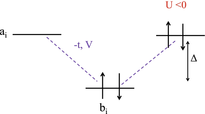
Schematic picture of an effective model Eq. (11). a site is Bi ion, and b site is oxygen ion

 Full size image 

where \(\tilde {t}=t^{2}/|\Delta |, \tilde {U}=U, \tilde {V}=zV|t/\Delta |^{2}\), with z being the number of nearest neighbor sites, and the hopping occurs between nearest neighbor sites a_i and \(a_{i+{2 \delta }}\) with the renormalized transfer integral \({\tilde t}\).

With the use of the canonical transformation [14, 15]

\(\begin{array}{@{}rcl@{}} c_{a_{i}\uparrow} &\rightarrow& {\tilde c}_{a_{i}\uparrow}, \end{array}\)

(12)

\(\begin{array}{@{}rcl@{}} c_{a_{i}\downarrow} &\rightarrow& P_{a_{i}} {\tilde c}_{a_{i}\downarrow}^{\dagger}, \end{array}\)

(13)

where \(P_{a_{i}} = 1\) (a_i∈A site) and \(P_{a_{i}} =-1\) (a_i∈B site), the hopping term is transformed as

\(-{\tilde t}\left(c^{\dagger}_{a_{i}\uparrow}c_{a_{i+2\delta}\uparrow} +c^{\dagger}_{a_{i}\downarrow}c_{a_{i+2\delta}\downarrow}\right) \rightarrow -{\tilde t}\left({\tilde c}^{\dagger}_{a_{i}\uparrow}{\tilde c}_{a_{i+2\delta}\uparrow} -{\tilde c}^{\dagger}_{a_{i}\downarrow}{\tilde c}_{a_{i+2\delta}\downarrow}\right).\)

(14)

Similarly, the number of electrons are mapped to the z-component of spin as

\(\begin{array}{@{}rcl@{}} n_{a_{i}} &=& c_{a_{i}\uparrow}^{\dagger}c_{a_{i}\uparrow} + c_{a_{i}\downarrow}^{\dagger}c_{a_{i}\downarrow} \\ &\rightarrow& {\tilde c}_{a_{i}\uparrow}^{\dagger}{\tilde c}_{a_{i}\uparrow} - {\tilde c}_{a_{i}\downarrow}^{\dagger}{\tilde c}_{a_{i}\downarrow} +1, \\ &=&2S_{a_{i}}^{z} +1. \end{array}\)

(15)

Then, \(n_{a_{i}\uparrow }n_{a_{i}\downarrow }\) is transformed as

\(\begin{array}{@{}rcl@{}} n_{a_{i}\uparrow}n_{a_{i}\downarrow} &=& a_{{i}\uparrow}^{\dagger}c_{a_{i}\uparrow}+c_{a_{i}\downarrow}^{\dagger}c_{a_{i}\downarrow} \\ &\rightarrow& {\tilde c}_{a_{i}\uparrow}^{\dagger}{\tilde c}_{a_{i}\uparrow}{\tilde c}_{a_{i}\downarrow}^{\dagger}{\tilde c}_{a_{i}\downarrow} \\ &=&-{\tilde n}_{a_{i}\uparrow}{\tilde n}_{a_{i}\downarrow} +\frac{1}{2}\left({\tilde n}_{a_{i}}-S_{a_{i}}^{z}\right). \end{array}\)

(16)

Therefore, the effective Hamiltonian Eq. (11) is mapped to the model with the repulsive-U Coulomb interaction:

\(\begin{array}{@{}rcl@{}} \tilde{H} &=& - \tilde{t}\sum\limits_{i,\delta,\sigma}{\tilde c}_{a_{i}\sigma}^{\dagger}{\tilde c}_{a_{i+2\delta}\sigma} + |\tilde{U}|\sum\limits_{i}{\tilde n}_{a_{i}\uparrow}{\tilde n}_{a_{i}\downarrow} \\ & & + \tilde{V} \sum\limits_{i,\delta}S_{a_{i}}^{z}S_{a_{i+2\delta}}^{z} + h \sum\limits_{i}S_{a_{i}}^{z} -{\tilde \mu}\sum\limits_{i}{\tilde n}_{a_{i}}, \end{array}\)

(17)

where \(h{\equiv }\tilde {\mu } + |\tilde {U}|/2 -2z\tilde {V}\), and \({\tilde \mu }\equiv |\tilde {U}|/2\).

In the case \(|\tilde {U}| \gg \tilde {t}, |\tilde {U}| \gg \tilde {V}\), the Hamiltonian Eq. (17) is further approximated by the anisotropic Heisenberg model as follows:

\(\begin{array}{@{}rcl@{}} \tilde{H} = \tilde{J}\sum\limits_{i,\delta}\boldsymbol{S}_{a_{i}} \cdot \boldsymbol{S}_{a_{i+2\delta}} + \tilde{V}\sum\limits_{i,\delta}{S}_{a_{i}}^{z} \cdot {S}^{z}_{a_{i+2\delta}}+h \sum\limits_{i}S_{a_{i}}^{z}, \end{array}\)

(18)

where \(\tilde {J}\simeq 4\tilde {t}^{2}/|U|\).

By the unitary transformation Eqs. (12) and (13), the Cooper pair’s operator is mapped to \(S_{a_{i}}^{+}, S_{a_{i}}^{-}\) as

\(\begin{array}{@{}rcl@{}} c_{a_{i}\uparrow}^{\dagger}c_{a_{i}\downarrow}^{\dagger} &\rightarrow& P_{a_{i}} {\tilde c}_{a_{i}\uparrow}^{\dagger} {\tilde c}_{a_{i}\downarrow} = P_{a_{i}}S_{a_{i}}^{+}, \end{array}\)

(19)

\(\begin{array}{@{}rcl@{}} c_{a_{i}\downarrow}^{\dagger}c_{a_{i}\uparrow}^{\dagger} &\rightarrow& -P_{a{i}} {\tilde c}_{a_{i}\downarrow}^{\dagger} {\tilde c}_{a_{i}\uparrow} = - P_{a_{i}}S_{a_{i}}^{-}. \end{array}\)

(20)

Therefore, the xy-antiferromagnetic state in the mapped world corresponds to the s-wave superconductivity in the original physical world. On the other hand, the Ising-antiferromagnetic state in the mapped world corresponds to the charge ordered state, considering the relation Eq. (15). The effect of the external magnetic field h in the mapped world has the effect of the carrier doping δ in the original physical world because the relation \(\langle \sum _{i}S^{z}_{a_{i}}\rangle =\langle \sum _{i}(n_{a_{i}}-1)/2\rangle\) according to the relation Eq. (15).

The phase diagram of the effective Hamiltonian Eq. (18) is calculated by the mean-field approximation as shown in Fig. 4 [2]. In the low magnetic field region, \(h\lesssim (2{\tilde V}{\tilde J}+{\tilde V}^{2})^{1/2}\), the Ising-antiferromagnetic state, where the staggered z-component of spins order, is stabilized, while the xy-antiferromagnetic state with staggered component in the xy plane is stabilized in the intermediate magnetic field region \((2{\tilde V}{\tilde J}+{\tilde V}^{2})^{1/2}{\lesssim } h \lesssim ({\tilde J}+{\tilde V})\). Here, the latter condition is to avoid the fully polarized ferromagnetic state. Therefore, the phase diagram shown in Fig. 4 can be interpreted in the original physical world as follows. Near half filling (δ∼0), the charge ordered insulating state occurs, and the s-wave superconducting state appears by the carrier doping (δ>δ^∗). This result well captures a global character of the phase diagram observed in Ba _1−xK_xBiO₃ [16].

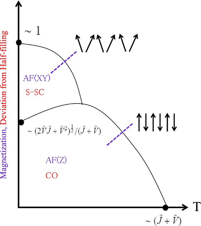
Phase diagrams of Eq. (18) based on the mean field approximation [2]. AF(XY), AF(Z), S-SC, and CO indicate the antiferromagnetic state with staggered component in the xy plane, Ising-antiferromagnetic state with the staggered z-component of spins order, s-wave superconducting state, and the charge ordered state, respectively. Blue (red) character means the mapped (original physical) world

 Full size image 

The effective Hamiltonian Eq. (11) is valid for the case where the hopping of electrons occurs only between the nearest neighbor sites in the bipartite lattice which are divided into two sublattices, with A and B sites. If the hopping is allowed between the next nearest neighbor sites and/or lattice points cannot be divided into two sublattices, e.g., triangular lattice, the fictitious magnetic field arises from the term of electron hopping in the mapped world by the transformation, Eqs. (12) and (13), even if in the half-filling. Indeed, the hopping between the nearest neighbor sites a_i and \(a_{i+{\delta }^{\prime }}\) is transformed as

\(-t^{\prime}\sum\limits_{i,{\delta^\prime}}\left(c^{\dagger}_{a_{i}\uparrow}c_{a_{i+{\delta}^{\prime}}\uparrow} +c^{\dagger}_{a_{i}\downarrow}c_{a_{i+{\delta}^{\prime}}\downarrow}\right) \rightarrow -t^{\prime}\sum\limits_{i,{\delta}^\prime}\left({\tilde c}^{\dagger}_{a_{i}\uparrow} {\tilde c}_{a_{i+{\delta}^{\prime}}\uparrow} -{\tilde c}^{\dagger}_{a_{i}\downarrow}{\tilde c}_{a_{i+{\delta}^{\prime}}\downarrow}\right),\)

(21)

which implies that there exists a wave-number dependent magnetic field in the mapped world. Namely, the hopping between the next nearest neighbor has an effect equivalent to the carrier doping which favors the appearance of the s-wave superconductivity. Therefore, the s-wave superconductivity might be induced by applying pressure on the charge ordered insulator. One of possible candidates is Na _1/3VO₂ [17], assuming that vanadium (V) is also the valence skipping element.

Charge Kondo effect based on negative-U effect

The charge Kondo effect based on the Anderson model with the negative-U interaction has been discussed especially in Refs. [18,19,20]. Since this effective model is deeply related with Tl-doped PbTe, we describe the details in Sec. 4.2.

The 5s or 6s wave function of the valence skippers such as Tl ion and Bi ion is extending comparing from the 3d and 4f orbitals. Thus, it is expected that the Coulomb interaction between s orbital and conduction band is important to understand the origin of the valence skipping phenomenon. Here, on the basis of the pair hopping interaction which is one of the Coulomb interactions between s electron and conduction electron, the origin of the valence skipping, the charge Kondo effect, and the superconductivity are discussed [4, 21]. Therefore, in this section, we give an introduction to the valence skipping phenomena based on the pair hopping interaction.

Unified theory of valence skip and charge Kondo effect based on the pair hopping interaction

An effective model including the coulomb interaction between the conduction electron and 5s (or 6s) orbital is given as

\(\begin{array}{@{}rcl@{}} \mathcal{H}_{0} = \mathcal{H}_{\mathrm{c}}+\mathcal{H}_{\mathrm{d}} + \mathcal{H}_{\text{dc}} + \mathcal{H}_{\text{ph}}, \end{array}\)

(22)

where the first term is the conduction electron, the second term is one-body term of 5s (6s) orbital (denoted by d hereafter), and the third and forth terms are the Coulomb interactions and that of pair hopping between conduction electron and s orbital. These terms are given as

\(\begin{array}{@{}rcl@{}} \mathcal{H}_{\mathrm{c}}& \equiv& \sum\limits_{\boldsymbol{k}\sigma}(\epsilon_{\boldsymbol{k}} -\mu) c_{\boldsymbol{k}\sigma}^{\dagger}c_{\boldsymbol{k}\sigma}, \end{array}\)

(23)

\(\begin{array}{@{}rcl@{}} \mathcal{H}_{\mathrm{d}} &\equiv& (\Delta_{\mathrm{d}} -\mu)\sum\limits_{\sigma} n_{\mathrm{d}\sigma}, \end{array}\)

(24)

\(\begin{array}{@{}rcl@{}} \mathcal{H}_{\text{dc}} &\equiv& U_{\text{dc}} \sum\limits_{\boldsymbol{k} \sigma\sigma^{\prime}} c_{\boldsymbol{k}\sigma}^{\dagger}c_{\boldsymbol{k}^{\prime} \sigma}n_{\mathrm{d}\sigma^{\prime}}, \end{array}\)

(25)

\(\begin{array}{@{}rcl@{}} \mathcal{H}_{\text{ph}} &\equiv& J_{\text{ph}}\sum\limits_{\boldsymbol{k} \boldsymbol{k}^{\prime}} \left[ d_{\uparrow}^{\dagger}d_{\downarrow }^{\dagger} c_{\boldsymbol{k}^{\prime}\downarrow} c_{\boldsymbol{k}\uparrow}+\text{h.c.} \right]. \end{array}\)

(26)

Since we focus on the charge degree of freedom, we introduce the following pseudo spins:

\(\begin{array}{@{}rcl@{}} I^{z}_{\mathrm{d}} &\equiv& \frac{1}{2} (n_{\mathrm{d}\uparrow} + n_{\mathrm{d}\downarrow} -1), \end{array}\)

(27)

\(\begin{array}{@{}rcl@{}} I^{+}_{\mathrm{d}} &\equiv& d_{\uparrow}^{\dagger}d_{\downarrow}^{\dagger}, \end{array}\)

(28)

\(\begin{array}{@{}rcl@{}} I^{-}_{\mathrm{d}} &\equiv& d_{\downarrow}d_{\uparrow}, \end{array}\)

(29)

and the pseudo spins corresponding to the conduction electron are

\(\begin{array}{@{}rcl@{}} I^{z}_{\mathrm{c}} &\equiv& \frac{1}{2} \sum\limits_{\boldsymbol{k} \boldsymbol{k}^{\prime}}\left(c_{\boldsymbol{k}\uparrow}^{\dagger}c_{\boldsymbol{k}^{\prime}\uparrow} + c_{\boldsymbol{k}\downarrow}^{\dagger}c_{\boldsymbol{k}^{\prime}\downarrow} -\delta_{\boldsymbol{k}\boldsymbol{k}^{\prime}}\right), \end{array}\)

(30)

\(\begin{array}{@{}rcl@{}} I^{+}_{\mathrm{c}} &\equiv& \sum\limits_{\boldsymbol{k}\boldsymbol{k}^{\prime}}c_{\boldsymbol{k}\uparrow}^{\dagger}c_{\boldsymbol{k}^{\prime}\downarrow}^{\dagger}, \end{array}\)

(31)

\(\begin{array}{@{}rcl@{}} I^{-}_{\mathrm{c}} &\equiv& \sum\limits_{\boldsymbol{k}\boldsymbol{k}^{\prime}}c_{\boldsymbol{k}\downarrow}c_{\boldsymbol{k}^{\prime}\uparrow}. \end{array}\)

(32)

Using these pseudo spins, the effective Hamiltoninan \(\mathcal {H}_{0}\) is mapped to

\(\begin{array}{@{}rcl@{}} \mathcal{H}_{0} \rightarrow \tilde{\mathcal{H}}_{0} =\tilde{\mathcal{H}}_{\mathrm{c}} + \tilde{\mathcal{H}}_{\text{pot}} + \tilde{\mathcal{H}}_{\text{dc}} + \tilde{\mathcal{H}}_{\text{ph}} + \tilde{\mathcal{H}}_{\mathrm{d}}, \end{array}\)

(33)

where

\(\begin{array}{@{}rcl@{}} \tilde{\mathcal{H}}_{\mathrm{c}}&\equiv& \sum\limits_{\boldsymbol{k}\sigma}\left(\epsilon_{\boldsymbol{k}} -\mu +U_{\text{dc}}\right) c_{\boldsymbol{k}\sigma}^{\dagger}c_{\boldsymbol{k}\sigma}, \end{array}\)

(34)

\(\begin{array}{@{}rcl@{}} \tilde{\mathcal{H}}_{\text{pot}}&\equiv& \sum\limits_{\boldsymbol{k}\boldsymbol{k}^{\prime} (\boldsymbol{k} \neq \boldsymbol{k}^{\prime})} U_{\text{dc}}c_{\boldsymbol{k}\sigma}^{\dagger}c_{\boldsymbol{k}^{\prime}\sigma}, \end{array}\)

(35)

\(\begin{array}{@{}rcl@{}} \tilde{\mathcal{H}}_{\text{dc}} &\equiv& 4U_{\text{dc}}I^{z}_{\mathrm{d}}I^{z}_{\mathrm{c}}, \end{array}\)

(36)

\(\begin{array}{@{}rcl@{}} \tilde{\mathcal{H}}_{\text{ph}} &\equiv& J_{\text{ph}}\left(I^{+}_{c}I^{-}_{\mathrm{d}} + I^{-}_{\mathrm{c}}I^{+}_{\mathrm{d}}\right), \end{array}\)

(37)

\(\begin{array}{@{}rcl@{}} \tilde{\mathcal{H}}_{\mathrm{d}} &\equiv& 2\left(\Delta_{\mathrm{d}} -\mu +U_{\text{dc}}\right)I_{\mathrm{d}}^{z}. \end{array}\)

(38)

\(\tilde {\mathcal {H}}_{\text {pot}}\) and \(\tilde {\mathcal {H}}_{\mathrm {d}}\) are the terms of the potential scattering and effective magnetic field to the pseudo spin, while we find that the others are mapped to the anisotropic Kondo model.

To understand the role of the pair hopping term Eq. (36), using a simple parameter setting, we calculate the temperature dependence of the entropy (S_imp) and the number of electrons (Q_d) in s orbital on the basis of numerical renormalization group. As shown in Fig. 5, we find that the valence skipping state appears as the temperature decreases because the existence of Q_d=1 is zero, and the charge Kondo-Yosida singlet state occurs at the low temperature (S_imp/ ln2→0). Therefore, we can understand the valence skip and charge Kondo effect unifiedly on the basis of the pair hopping interaction.

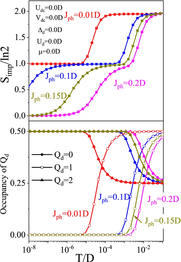
Temperature dependence on the entropy in the impurity site (S_imp), and temperature depenedence on number of electrons (Q_d) [4]

 Full size image 

In the realistic system, the hybridization between the s-electron and the conduction band is an essential role to a ground state. Therefore, we suggest the general and realistic model given by

\(\begin{array}{@{}rcl@{}} \mathcal{H} = \mathcal{H}_{0} + \mathcal{H}_{\mathrm{U}}+ \mathcal{H}_{\text{hyb}}, \end{array}\)

(39)

where the second term is the Coulomb interaction on s orbital site, and the third term is the hybridization between conduction band and s orbital, and these terms are written as

\(\begin{array}{@{}rcl@{}} \mathcal{H}_{\mathrm{U}}&\equiv& U_{\mathrm{d}}n_{\mathrm{d}\uparrow}n_{\mathrm{d}\downarrow}, \end{array}\)

(40)

\(\begin{array}{@{}rcl@{}} \mathcal{H}_{\text{hyb}}&\equiv& V_{\text{dc}}\sum\limits_{\boldsymbol{k},\sigma} \left(c_{\boldsymbol{k},\sigma}^{\dagger}d_{\sigma} +\text{{h.c}}\right). \end{array}\)

(41)

As discussed above, for V_dc=0 and U_d=0, the ground state is the charge Kondo-Yosida singlet state, while as V_dc increases, the spin and charge degrees of freedom mix, and for the strong hybridization and the finite U_d, it is expected that the ground state is the usual Kondo-Yosida singlet state.

Figure 6 shows the hybridization and temperature dependence of entropy in the impurity site. The parameter settings and the details see ref. [4].

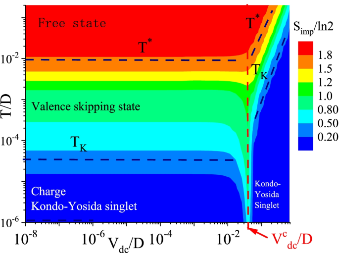
Temperature and hybridization dependence on the entropy of impurity site

 Full size image 

As a result, for the small hybridization, the Kondo temperature T_K is independent of the amplitude of hybridization, and the ground state is mainly the charge degree of freedom. For the large hybridization, the ground state is the mixing state of charge and spin degrees of freedom such as usual Kondo-Yosida singlet. On the other hand, in the middle region (\(V_{\text {dc}} \sim V_{\text {dc}}^{\mathrm {c}}\)), it is found that the Kondo temperature decreases drastically and the residual entropy is k_Bln2 until the low temperature. This origin is expected to be the competition between pair hopping and hybridization.

Possibility of superconductivity caused by pair-hopping interaction

In this subsection, we discuss how the pair-hopping interaction works to stabilize the superconductivity in the lattice system. According to the discussion in Section 3.1, the pair-hopping interaction causes the negative U effect, leading to the charge Kondo effect at the impurity level. Therefore, it is reasonable to expect that the pair-hopping interaction promote the superconductivity also in the lattice system. Indeed, Kondo discussed two decades ago that the pair-hopping interaction causes the superconductivity in a two-band electron system with only repulsive interaction among electrons even though enhancement of the pairing-hopping interaction by charge Kondo effect is not taken into account [21]. Let us briefly recapitulate an essential point of Kondo theory.

Kondo started by classifying the Coulomb interaction in the two-band (1 and 2) representation and focus on the intraband Coulomb repulsion U₁ and U₂, and the pair-hopping interaction K, which corresponds to J_ph in Eq. (26) or Eq. (37). Namely, the model Hamiltonian H_pair, which is essentially equivalent to that treated by Kondo [21], is given as

\(\begin{array}{@{}rcl@{}} & &H_{\text{pair}}=\sum\limits_{m=1,2}\left[\sum\limits_{\boldsymbol{k},\sigma}\xi_{m}(\boldsymbol{k}) c^{\dagger}_{m\boldsymbol{k}\sigma}c_{m\boldsymbol{k}\sigma} \right. \\ & &\qquad\qquad\qquad \left. +U_{m}\sum\limits_{\boldsymbol{k},\boldsymbol{k}^{\prime}}c^{\dagger}_{m\boldsymbol{k}\uparrow}c^{\dagger}_{m,-\boldsymbol{k}\downarrow} c_{m,-\boldsymbol{k}^{\prime}\downarrow}c_{m\boldsymbol{k}^{\prime}\uparrow}\right] \\ & &\qquad\quad +{\tilde K}\sum\limits_{\boldsymbol{k},\boldsymbol{k}^{\prime}}\left(c^{\dagger}_{1\boldsymbol{k}\uparrow} c^{\dagger}_{1,-\boldsymbol{k}\downarrow} c_{2,-\boldsymbol{k}^{\prime}\downarrow}c_{2\boldsymbol{k}^{\prime}\uparrow}+\text{h.c.}\right), \end{array}\)

(42)

where m = 1,2 are band index, ξ_m(k) is band dispersion of band m, U_m is the intraband Coulomb interaction, and \({\tilde K}=zK\), with z being the number of nearest neighbor sites, is the pair-hopping interaction among bands m=1 and m = 2. The linearized and coupled gap equations determining the transition temperature T_c are given by extending mean field approximation of BCS theory as follows:

\(\begin{array}{@{}rcl@{}} & &\Delta_{1}=-U_{1}\Phi_{1}(T_{\mathrm{c}})\Delta_{1}-{\tilde K}\Phi_{2}(T_{\mathrm{c}})\Delta_{2}, \end{array}\)

(43)

\(\begin{array}{@{}rcl@{}} & &\Delta_{2}=-U_{2}\Phi_{2}(T_{\mathrm{c}})\Delta_{2}-{\tilde K}\Phi_{1}(T_{\mathrm{c}})\Delta_{1}, \end{array}\)

(44)

where Δ_m represents the superconducting gap of band m, the function Φ_m(T) is defined by

\(\Phi_{m}(T)\equiv\sum\limits_{\boldsymbol{k}}\frac{\text{tanh}[\xi_{m}(\boldsymbol{k})/2T]}{2\xi_{m}(\boldsymbol{k})}.\)

(45)

From the condition for coupled Eqs. (43) and (44) to have non-trivial solution, the transition temperature T_c is determined by solving the following equation:

\(1+\sum\limits_{m=1,2}U_{m}\Phi_{m}(T_{\mathrm{c}})+ \left(U_{1}U_{2}-{\tilde K}^{2}\right)\Phi_{1}(T_{\mathrm{c}})\Phi_{2}(T_{\mathrm{c}})=0.\)

(46)

In the low temperature region T≪D_m,D_m being half the band width of band m, Φ_m(T)∝− log(T/D_m) so that the condition for Eq. (46) has the solution T_c>0 is given by

\({\tilde K}^{2}>U_{1}U_{2}.\)

(47)

If this condition is fulfilled, s-wave superconductivity appears at T<T_c.

It is crucial to note that the cut-off energy ω_c appearing in the definition of Φ_m(T) Eq. (45) is given by D_m because the summation over k extends to the whole band, so that ω_c is far larger than the Debye energy ω_D appearing in the BCS theory based on electron-phonon mechanism. Therefore, this superconducting mechanism has the potential causing high superconducting transition temperature T_c.

However, it seems rather hard to satisfy the condition (47) in a conventional situation, while Kondo argued that the increase of number of nearest neighbor site z can support to fulfill the condition (47) even in the 3d electron systems [21]. On the other hand, \({\tilde K}\lesssim U_{m}\) (m = 1,2) is expected in the elements with the large principle quantum number ns (n = 4−6). Furthermore, due to the many-body effect associated with the charge Kondo effect, the renormalized pair-hopping interaction K (which is equivalent to J_ph grows logarithmically in the low energy region and works cooperatively to promote the realization of superconductivity. In other words, this implies that the mechanism of superconductivity can be discussed even without sorting to the negative-U effect discussed in Section 2. However, since the discussion there is only for the impurity model, we need further studies to obtain a comprehensive picture for the superconductivity promoted by the pair-hopping interaction.

Recently, by analyzing the lattice model with the pair hopping interaction J_ph and the Coulomb interaction (U^′) between the conduction electron and localized state (extended Falikov-Kimball model) based on the continuous time quantum Monte Carlo method, it was clarifed that the charge Kondo-Yosida single state survives even at zero temperature and this state competes with the charge ordered state and s-wave superconducting state [22].

Experimental facts suggesting charge-Kondo effect

In this subsection, we review the experimental results on Tl-doped PbTe that exhibits superconductivity and Kondo-like effect, which is one of the promising candidates for novel superconducting (SC) mechanism related to the valence skipping phenomena [3, 5, 23,24,25,26,27].

PbTe is a narrow-gap semiconductor. A small amount of substitution of Tl for Pb (i.e., Pb _1−xTl_xTe) leads to an SC ground state when x exceeds x_c∼0.3%, as shown in Fig. 7(a) [3, 23,24,25]. Significantly, Tl is the only dopant known to cause superconductivity in PbTe, suggesting that these specific impurities have a unique effect on the electronic states near the Fermi energy. Although the carrier densities are ≲10²⁰cm⁻³, the SC transition temperature rises to T_c∼1.5 K for x∼1.5% (the solubility limit), which is higher than that of other well-known low-carrier-density superconductors, such as SrTiO₃ [28]. As shown in Fig. 7(b) [3, 20, 24, 29], the hole density p, estimated by Hall coefficient measurements, increases linearly with x for compositions up to x∼x_c, implying that each Tl impurity acts as an acceptor, having a formal valence Tl ¹⁺. However, as x increases further, the increase in p gradually saturates, implying that impurities no longer contribute one hole per dopant. Drawing on the known valence-skipping character of Tl ions [2], this behavior has been interpreted in terms of the onset of a degeneracy of impurity states with a formal valence of Tl ¹⁺(hole doping) and Tl ³⁺(electron doping) for x>x_c [3, 24, 25, 30]. Recently, the detail of Fermi surface has been discussed by the magnetotransport measurements [31]. It should be noted that, although there are several experimental reports on the electronic state and charge state of Tl-doped PbTe [32, 33], there is no direct evidence of the charge fluctuation under the pinning of the chemical potential. It is expected to be observed in the future. As shown in Fig. 7(c) [3, 23,24,25, 34], the indirect support for such a scenario was obtained via the observation of a logarithmic upturn in the resistivity at low temperatures for x>x_c, reminiscent of the Kondo effect [35], but in the absence of unpaired spins [3, 36]. Since the − logT behavior of the resistivity is not affected by the magnetic field [3], it is suggested that the Kondo-like effect is different from the usual Kondo effect whose origin is due to the magnetic degrees of freedom of impurity. This observation was interpreted as evidence for a charge Kondo effect, that is, a Kondo effect arising from the interaction of the conduction electrons with the two degenerate valence states of the Tl dopants [3, 4, 19, 20, 29, 37]. The fact that such an effect is observed only for SC compositions (x>x_c) [3, 38] implies that valence fluctuations might play a key role in the pairing interaction in Pb _1−xTl_xTe, possibly explaining the high critical temperatures found in this system [2, 4, 19, 20, 29, 37].

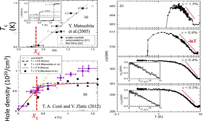
a Superconducting phase diagram of Pb _1−xTl_xTe [3]. Inset shows representative resistivity data for single crystals. b Hole density vs. Tl doping x for T = 1.8 K and 77 K, obtained experimentally [3, 24] and theoretically [29]. c Temperature dependence of the resistivity for Pb _1−xTl_xTe [3, 34]. A logarithmic upturn is observed in the resistivity at low temperatures only for x>x_c, reminiscent of the Kondo effect [35], but in the absence of unpaired spins [3, 34, 36]. Adapted from [3] for Fig. 7a and Fig. 7c and from [29] for Fig. 7b

 Full size image 

To understand behaviors presented in Fig. 7a and c more precisely, the following two aspects should be considered: First of all, there are two contributions to the resistivity, one form the charge Kondo effect and the others from the normal processes consisting of normal electron-electron and electron-phonon scatterings. Therefore, the increasing tendency of the resistivity with decreasing temperature (due to the charge Kondo effect) is compensated by its decreasing tendency (due to the above two normal scatterings), so that we should be careful in estimating T_K from the raw data of the temperature dependence of resistivity. The observed temperature range (T<10K) shown in Fig. 7c does not seem to be wide enough to draw a definite conclusion for the concentration dependence of T_K predicted by Eq. (54). Secondly, the superconducting transition temperature T_c shown in Fig. 7a is determined both by the effective Fermi energy \(E^{*}_{\mathrm {F}}\) (which depends crucially on the Tl’s concentration), and the pairing interaction V_pair (which is essentially given by the on-site effect). As a result, the two phenomena exhibit different response to the doping.

Recently, a piece of direct spectroscopic evidence of the skipping of Tl ²⁺ state in Pb _1−xTl_xTe was reported [39]. On the other hand, the Kondo like anomalies in the resistivity have been reported since early 1980’s in a series of compounds Pb _1−xGe_xTe [40], Pb _1−xTl_xTe [32], and Pb _1−xGe_xSe [41], although such anomalies have been interpreted essentially as the so-called two-level Kondo effect due to the bi-stable position of constitute ions [42].

Theoretical description of charge Kondo effect and superconductivity

From theoretical point of view, a possibility of the charge Kondo effect has already been proposed a quarter century ago on the basis of negative-U Anderson model as [19]

\(H =\sum\limits_{\boldsymbol{k}\sigma}(\epsilon_{\boldsymbol{k}} -\mu)c_{\boldsymbol{k}\sigma}^{\dagger}c_{\boldsymbol{k}\sigma} + \sum\limits_{\boldsymbol{k}j\sigma}V(c_{\boldsymbol{k}}^{\dagger}d_{j\sigma}e^{i\boldsymbol{k}\cdot\boldsymbol{R}_{j}} +h.c.) + \sum\limits_{j}\left[\left(E_{\mathrm{d}} -\mu+\frac{U}{2}\right)n_{j\mathrm{d}} +\frac{U}{2}(n_{j\mathrm{d}} -1)^{2} \right],\)

(48)

where d_j is an annihilation operator at j-site, and U is a negative. The equivalence of this Hamiltonian to the conventional Anderson model can be understood from the identity

\(\left(d^{\dagger}_{i\uparrow}d_{i\uparrow}+d^{\dagger}_{i\downarrow}d_{i\downarrow}-1\right)^{2} =1-d^{\dagger}_{i\uparrow}d_{i\uparrow}-d^{\dagger}_{i\downarrow}d_{i\downarrow} +2d^{\dagger}_{i\uparrow}d_{i\uparrow}d^{\dagger}_{i\downarrow}d_{i\downarrow}.\)

(49)

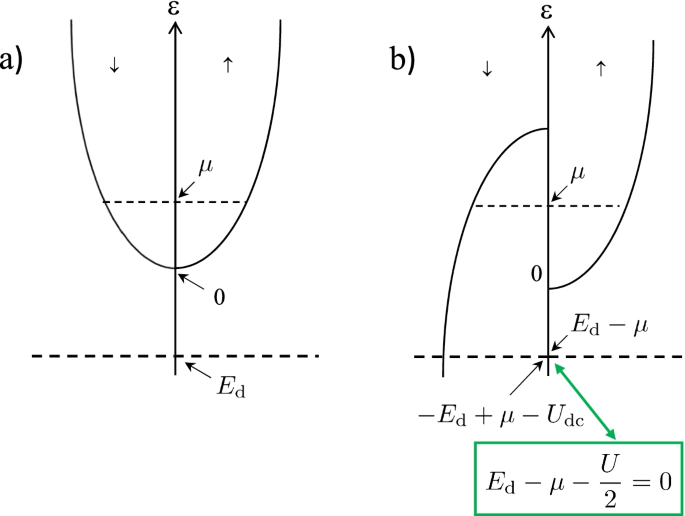
The doping of Tl to PbTe makes the chemical potential μ be increased from the bottom of conduction band of PbTe. When the chemical potential reaches μ = E_d +(U/2), the last term in Eq. (48) takes degenerate tow minimum U/2<0, i.e., the number of electrons on 6s orbital, n_d, takes two values, n_d = 0 or n_d = 2. Since the two states are degenerate at this chemical potential, the chemical potential is pinned at μ=E_d+(U/2) even though the carriers are doped on 6s orbital, as shown in Fig. 8. This means that when at μ=E_d +U/2 electrons are doped in this system, the doped electrons fill the 6s orbital until the 6s orbital is completely filled. In this sense, the degeneracy of the states, n_d = 0 and n_d = 2, is not accidental but inevitable.

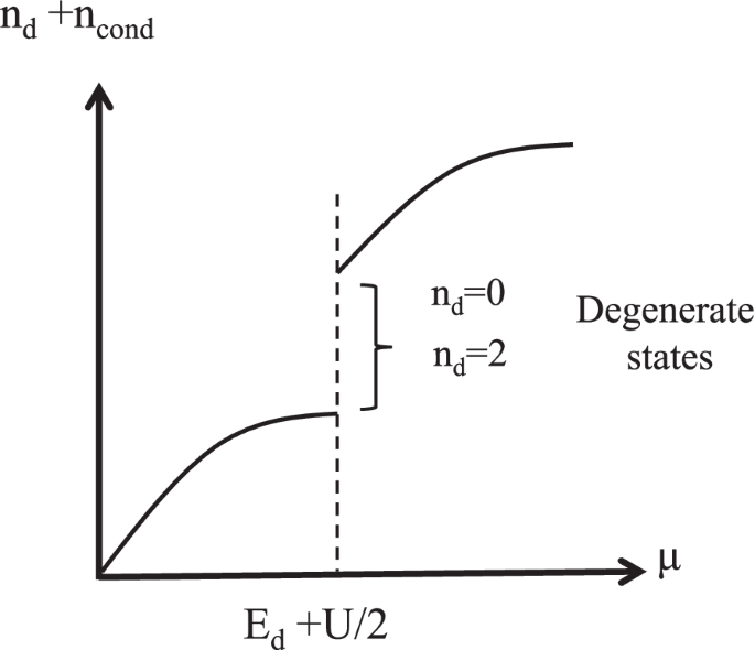
Number of electron and chemical potential

 Full size image 

The Hamiltonian (48) is mapped to the repulsive Anderson model by the canonical transformation

\(\begin{array}{@{}rcl@{}} d_{j\downarrow}^{\dagger} &\rightarrow& -{\tilde d}_{j\downarrow} \end{array}\)

(50)

\(\begin{array}{@{}rcl@{}} c_{\boldsymbol{k}\downarrow}^{\dagger} &\rightarrow& {\tilde c}_{-\boldsymbol{k}\downarrow}. \end{array}\)

(51)

Indeed, by the transformations, Eqs. (50) and (51), the Hamiltonian (48) is transformed to

\(\begin{array}{@{}rcl@{}} H &=& \sum\limits_{\boldsymbol{k}} \left[(\epsilon_{\boldsymbol{k}} -\mu){\tilde c}_{\boldsymbol{k}\uparrow}^{\dagger} {\tilde c}_{\boldsymbol{k} \uparrow} -(\epsilon_{\boldsymbol{k}} -\mu){\tilde c}_{\boldsymbol{k}\downarrow}^{\dagger} {\tilde c}_{\boldsymbol{k}\downarrow} \right] +\sum\limits_{\boldsymbol{k} j\sigma }V\left({\tilde c}_{\boldsymbol{k}}^{\dagger} {\tilde d}_{j\sigma}e^{i\boldsymbol{k}\cdot\boldsymbol{R}_{j}} +h.c.\right) \\ && + \sum\limits_{j}\left(E_{\mathrm{d}} -\mu -\frac{|U|}{2}\right){{\tilde m}}_{\mathrm{d}j} + \sum\limits_{j}\left[ -\frac{{|U|}}{2}{{\tilde n}}_{j\mathrm{d}} + {|U|}{{\tilde d}}_{j\uparrow}^{\dagger} {{\tilde d}}_{j\uparrow} {{\tilde d}}_{j\downarrow}^{\dagger} {{\tilde d}}_{j\downarrow} \right], \end{array}\)

(52)

where the dispersion of conduction electron is dependent on the spin of conduction electron, and the third term represents the effective Zeeman interaction acting on the impurity spin in the mapped world (magnetization is defined as \({\tilde m}\equiv \left ({\tilde d}_{j\uparrow }^{\dagger }{\tilde d}_{j\uparrow } -{\tilde d}_{j\downarrow }^{\dagger }{\tilde d}_{j\downarrow }\right)/2\)). Note that at μ=E_d−(|U|/2) (pinning condition), the third term is exactly zero, i.e., H=−[E_d−μ−(|U|/2)]=0.

In the case 0<E_d≪|U|, the Fermi level μ satisfies the condition, 0<μ≡E_d−(|U|/2)≪(|U|/2). Then, since the double occupancy on the impurity site is prohibited, the effective model is given by the Kondo-like model. It is crucial here that there still exist finite density of states (DOS) at the Fermi level, although the dispersion of conduction electrons with up-spin and down-spin components are opposite sign as shown in Fig. 9 for the density of states (DOS), Therefore, the Kondo effect can appear. By the canonical transformation, Eq. (51), the current density, \(\boldsymbol {j}=-e\sum _{\boldsymbol {k}\sigma }\boldsymbol {v}_{\boldsymbol {k}}c^{\dagger }_{\boldsymbol {k}\sigma }c_{\boldsymbol {k}\sigma }\), in the original physical world is transformed to the current density also in the mapped world. Indeed, the current j is transformed to \(\tilde {\boldsymbol {j}}\) as follows:

\(\begin{array}{@{}rcl@{}} \tilde{\boldsymbol{j}}&=&-e\sum\limits_{\boldsymbol{k}}\boldsymbol{v}_{\boldsymbol{k}} \left({\tilde c}^{\dagger}_{\boldsymbol{k}\uparrow}{\tilde c}_{\boldsymbol{k}\uparrow}+ {\tilde c}_{-\boldsymbol{k}\downarrow}{\tilde c}^{\dagger}_{-\boldsymbol{k}\downarrow}\right) \\ &=&-e\sum\limits_{\boldsymbol{k}}\boldsymbol{v}_{\boldsymbol{k}} \left({\tilde c}^{\dagger}_{\boldsymbol{k}\uparrow}{\tilde c}_{\boldsymbol{k}\uparrow}- {\tilde c}_{-\boldsymbol{k}\downarrow}{\tilde c}^{\dagger}_{-\boldsymbol{k}\downarrow}+1\right) \\ &=&-e\sum\limits_{\boldsymbol{k}\sigma}\boldsymbol{v}_{\boldsymbol{k}} {\tilde c}^{\dagger}_{\boldsymbol{k}\sigma}{\tilde c}_{\boldsymbol{k}\sigma}, \end{array}\)

(53)

a Schematic picture of the DOS for the original system and b that for the mapped world by the canonical transformations Eqs. (50) and (51)

 Full size image 

where we have assumed inversion symmetry, i.e., v_−k=−v_k. As a result, the Kondo effect appears both in the repulsive-U Anderson model and the negative-U Anderson model with μ=E_d−(|U|/2).

Next, we discuss the superconductivity based on negative-U Anderson model [20]. In the negative-U model, where the RKKY interaction between impurity spins is anisotropic. As temperature decreases, the RKKY interaction between spins in the xy plane I_±(R) increases in proportion to − logT, while that parallel to the z-axis I_z(R) exhibits only the usual Friedel oscillations. Therefore, the magnetic order in the xy plane sets in at T=T_c,T_c being the transition temperature. By the canonical transformation, Eq. (50), the magnetic state in the xy plane is mapped to the s-wave superconducting state due to the pair hopping of two electrons. This is because the spin operator \(S_{\mathrm {d}j}^{-}\), representing a spin flip from up-spin state to down-spin one, is transformed back to the spin-singlet Cooper pairing as \(S_{\mathrm {d}j}^{-}={\tilde d}_{j\downarrow }{\tilde d}_{j\uparrow } \rightarrow -d_{j\downarrow }^{\dagger }d_{j\uparrow }^{\dagger }\).

As well known in the usual Kondo lattice model, the competition between RKKY interaction and Kondo effect play a crucial role to determine the ground state. Namely, when the Kondo effect dominates the RKKY interaction, the magnetic state is suppressed, and vice versa. The doping (x) dependence of the Kondo temperature T_K and the energy scale of RKKY interaction T_RKKY are given as

\(\begin{array}{@{}rcl@{}} T_{\mathrm{K}}\sim x^{2/3}\exp\left(-\frac{a}{x^{1/3}J}\right), \end{array}\)

(54)

and

\(\begin{array}{@{}rcl@{}} T_{\text{RKKY}}\sim x^{1/3}R^{-3}J^{2}\sim x^{4/3}J^{2} \end{array}\)

(55)

where a is a constant with the dimension of energy. The exchange interaction J is given by J≃V²/(U−E_d), and the denstiy of states at the Fermi level is N_F∝x^1/3. In the dilute limit, x≪1,T_RKKY>T_K, so that the magnetic state in the repulsive-U model (s-wave superconducting state in the negative-U model) is stabilized.

As shown in the above discussions, the charge Kondo effect and the superconductivity in Tl-doped PbTe can be understood by the negative-U Anderson model. Namely, the origin of this charge Kondo effect is due to the degeneracy of the degenerate ionic states of 6s orbital of Tl ion, i.e., (6s)⁰ and (6s)², and the superconductivity is due to the negative-U effect, which is the origin of skipping (6s)¹ state. Costi et al. discussed the quantitative calculation by the numerical renormalization group calculation of the negative-U Anderson model with the realistic density of states [29].

Experimental results for anomaly of NMR relaxation rate 1/T ₁

Motivated by these bulk experiments and theoretical insights, the local electronic states around Tl dopants were investigated microscopically by means of NMR probes. In this subsection, we review ¹²⁵Te-NMR studies on Pb _1−xTl_xTe [5, 26, 27], revealing the unusual character of the local electronic states introduced by Tl dopants through systematic measurements of the Knight shift (K) and the nuclear spin relaxation rate (1/T₁T). Figure 10a shows the ¹²⁵Te-NMR spectra for x = 0, 0.35, and 1.0%. Here, the horizontal axis ΔK(x) is defined as K(x)−K(0) that represents the relative shift from that of x = 0. The full-width at half-maximum (FWHM) of the spectra increases with increasing x, as shown in the inset of Fig. 10a. The spectra composed by a single peak even in the doped samples indicate that the doped Tl atoms distribute randomly over the samples, excluding the presence of dopant clusters and/or decomposition. The doping of Tl atoms makes the ΔK(x) increase positively.

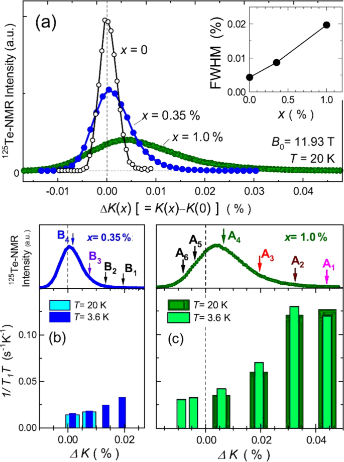
a ¹²⁵Te-NMR spectra at T = 20 K for x = 0, 0.35, and 1.0%. Here, the horizontal axis ΔK(x) is defined as K(x)−K(0) that represents the relative shift from that of x=0. Inset shows the x dependence of FWHM of the spectra represented in the scale of K(x). ¹²⁵Te-nuclear spin-lattice relaxation rate (1/T₁T) for b x = 0.35% and c x = 1.0% measured as a function of ΔK, corresponding to B _i(i = 1 to 4) and A _i(i = 1 to 6) denoted in the upper panels, respectively. The large (1/T₁T) at the large ΔK appears when x≠0 due to the presence of Tl dopants, since such anomaly is not observed in x = 0

 Full size image 

Generally, the observed K(x) comprises the spin shift K_s and the chemical shift K_chem. The former K_s is proportional to A_hfχ₀∝A_hfN₀, where A_hf is the hyperfine coupling constant, χ₀ is the static spin susceptibility at q = 0, and N₀(≡N_F) is the density of states (DOS) at the Fermi level (E_F). The ΔK(x)[≡K(x)−K(0)] corresponds to their spin components ΔK_s(x)[≡K_s(x)−K_s(0)], since K_chem is independent of x in a small range. Hence, the increase of ΔK(x) with Tl doping originates from the increase of χ₀ or N₀ at the Te sites in the vicinity of the Tl dopants. As shown in the inset of Fig. 10a, the FWHM in the spectrum is significantly increased toward positive side in ΔK(x) as increasing the number of Tl dopants, where the neighbor fraction of Te sites to the Tl dopants increases. Accordingly, the Te sites closer to the Tl dopants possess the larger ΔK_s(x) or the larger N₀ than those for the Te sites far from the Tl dopants.

Figure 10c shows the (1/T₁T) for x = 1.0% at T = 3.6 K and 20 K, which are measured at the Te sites denoted as A _i(i = 1 to 6) in the spectrum shown in the upper panel. Note that the values of ΔK are widely distributed over the sample, which allow us to examine each local electronic characteristics caused by the Tl dopants. In fact, the value of (1/T₁T) increases together with ΔK in contrast to a homogeneous value of 1/T₁ for the non-doped x = 0. It should be noted that the large values of (1/T₁T) associated with those of ΔK originate from the Te sites in the vicinity of the Tl dopants, indicative of some vital evolution in electronic state by doping Tl atoms. By contrast, such distributions at the Te sites denoted as B _i(i = 1 to 4) for x = 0.35% are significantly smaller than those for x = 1.0% as shown in Fig. 10b. Since such anomaly is not observed at x = 0, these results show that the presence of Tl dopants increases the distributions in (1/T₁T) and ΔK with increasing x. We emphasize that for x = 1.0% with T_c∼1.0 K, the (1/T₁T) are markedly enhanced at the near neighbor Te sites to the Tl dopants.

Remarkable feature of this compound was seen in the temperature (T) dependence of (1/T₁T), as presented in Fig. 11. In x = 0.35% (x≃x_c), (1/T₁T)= const. is observed at B₄ and B₃ in the T range of 1.4–60 K. In contrast, in x = 1.0% (x>x_c), the (1/T₁T) at A₁, A₂, and A₃ in the vicinity of the Tl dopants start to increase below \(T_{\text {min}}^{\text {NMR}}\simeq\)10 K. Note that \(T_{\text {min}}^{\text {NMR}}\simeq\)10 K coincides with the temperature below which the resistivity experiences a logarithmic upturn (\(T_{\text {min}}^{\rho }\) in the inset of Fig. 11) [3, 36]. By contrast, the (1/T₁T) at A₄ stays almost constant when the Te sites are located far from the Tl dopants. The observation of the logarithmic upturn in the resistivity below 10 K for x>x_c reminds us of the “spin” Kondo effect [21]. The difference from the spin Kondo effect is microscopically given by the facts that the static spin susceptibility χ₀ deduced from ΔK shows no apparent T dependence in the T range of 1.8 K <T<50 K, and the upturn in (1/T₁T) upon cooling below 10 K was not suppressed even in the application of the strong magnetic field ∼ 12 Tesla, which are consistent with the absence of spin-degree of freedom. Thus, our results may be related to the possible resonating valence state of two degenerate charge states of 2 e⁻(Tl ¹⁺) and 0 e⁻(Tl ³⁺), which has been theoretically accounted for by “charge” Kondo effect [2, 4, 19, 20, 29, 37] in analogy with two degenerate spin states in “spin” Kondo effect [35].

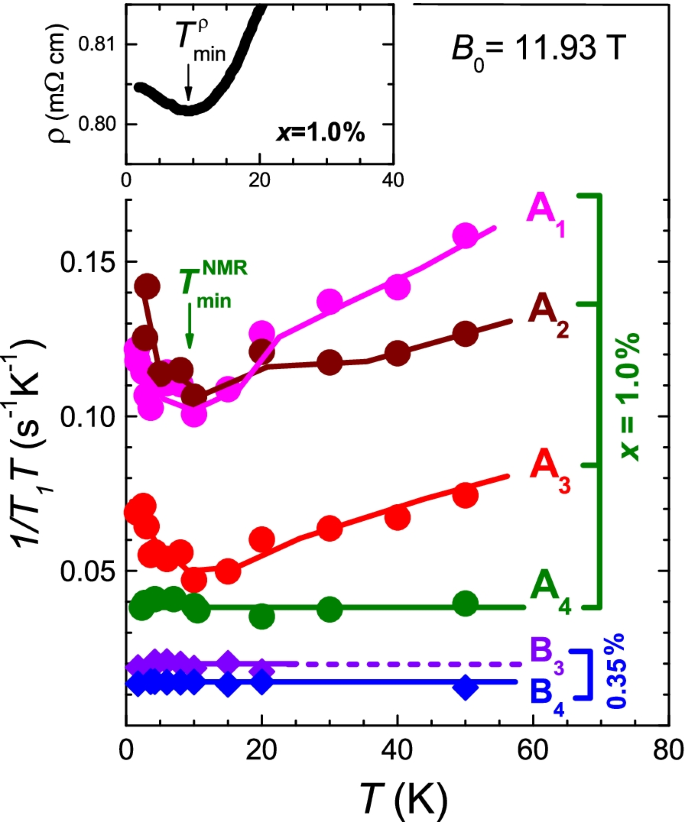
T dependence of (1/T₁T) for x=0.35 and x=1.0% measured at ΔK denoted as B _i and A _i in the upper panels of Fig. 10b and c, respectively. The anomalous increases of (1/T₁T) below \(T_{\text {min}}^{\text {NMR}}\sim\)10 K are seen only at A _i(i=1,2,3), corresponding to the Te sites close to Tl dopants in x=1.0%. Here, the \(T_{\text {min}}^{\text {NMR}}\) coincides with the temperature below which the resistivity shows upturn in the present sample (x= 1.0%) [3]. Inset shows the resistivity upturn below \(T_{\text {min}}^{\rho }\sim\)10 K observed in the present sample (x= 1.0%) [3]. Such anomaly was not seen in x=0.35% and 0%

 Full size image 

Figure 12 is schematic of possible distribution of the local electronic states of Tl-doped PbTe in the atomic scale, which are deduced from the present ¹²⁵Te-NMR study. Assuming that the Tl dopants occupy the Pb site and the lattice constant 6.46Å [43], the distance of Te sites from the Tl dopants are estimated for the 1st, 2nd, 3rd... nearest neighbor(NN) Te sites in the figure. The distance between the Tl dopants in average 〈d_Tl〉_av is roughly estimated to be ∼ 27 Å and ∼ 19 Å for x=0.35 and 1.0%, respectively. The solid curves in Fig. 12 represent the schematic spatial dependence of the local DOS N₀(r)^x deduced from ΔK_s, which becomes large at the near-neighbor Te sites to the Tl dopants. Here, the spatially averaged \(\langle N_{0}(r)\rangle _{\text {av}}^{x}\) are shown by the broken horizontal lines, which corresponds to spatially averaged \(\langle \Delta K_{\mathrm {s}}\rangle _{\text {av}}^{x}\), as shown in the inset. Since the wave function of the 6s orbital of the Tl dopants extends to near-neighbor Te sites around the Tl dopants [44, 45], we expect the strong hybridization between the 6s electrons at the Tl dopants and conduction electrons. In this context, we deduce that the coherent hopping of 6s-electron pairs may develop a Cooper-pairing formation below ∼ 1 K in Pb _1−xTl_xTe(x>x_c).

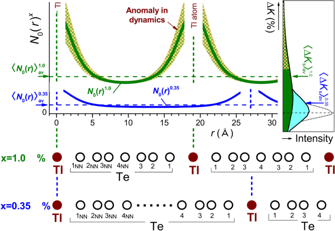
Schematic diagram illustrating the variation in local DOS N₀(r) deduced from our ¹²⁵Te-NMR study as a function of the distance (r) from a Tl dopant. The N₀(r)^x is enhanced locally around Tl dopants, which is deduced from the observed ΔK_s. The yellow/green hatched region indicates Te ions that exhibit an anomaly in the dynamical local electronic states as deduced from (1/T₁T) below 10 K. This effect is detected only for Te sites that are particularly close to Tl dopants for the SC sample with x = 1.0%(x≥x_c), whereas it is suppressed at Te sites far from Tl dopants and is not observed at all for the non-SC samples with x=0.35 and 0%. Here, the broken horizontal lines denote the spatially-averaged \(\langle N_{0}(r)\rangle _{\text {av}}^{x}\) that corresponds to spatially-averaged \(\langle \Delta K_{\mathrm {s}}\rangle _{\text {av}}^{x}\) in the right-hand inset

 Full size image 

In order to clarify the origin of an increase in (1/T₁T) in Tl-doped PbTe compounds, we performed the ¹²⁵Te-NMR study on the other hole-doped PbTe, that is a series of non-superconducting and non-valence skipping Na(Na ¹⁺)-doped PbTe. Figure 13a shows ¹²⁵Te-NMR spectra for x = 0, 0.46, and 1.45% in Pb _1−xNa_xTe, which is plotted as a function of K. The spectral broadening by doping Na impurities is observed in Na-doped PbTe compounds as well as in Tl-doped PbTe ones. The FWHM of ¹²⁵Te-NMR spectrum in Na-doped PbTe is plotted in the inset of Fig. 13a, together with that in Tl-doped PbTe. Both of them show a simlar linear positive relation with x, indicating that Na dopants are also randomly distributed in the crystals. The spectral peak position in Pb _1−xNa_xTe with x = 1.45% is more largely shifted to higher K than that in Pb _0.99Tl_0.01Te. The spectral broadening and peak shift to higher K suggests the large enhancement of local DOS surrounding each Na dopant in Pb _1−xNa_xTe with x = 1.45% as well as in Pb _0.99Tl_0.01Te. In the case of Tl-doped PbTe, two valence states of Tl ¹⁺(hole doping) and Tl ³⁺(electron doping) are degenerate for x>x_c (∼ 0.3%), leading to the suppression of carrier doping. However, Na is not a valence-skipping element. The increase in the hole concentration is not suppressed by Na doping with x>0.3%, since only Na ¹⁺ is doped into the Pb _1−xNa_xTe crystals. Thus, we suggest that the ¹²⁵Te-NMR spectrum in Pb _1−xNa_xTe with x = 1.45% is largely shifted to higher K than that in Pb _0.99Tl_0.01Te. The distributions in (1/T₁T) and K values by the Na impurities are also observed in the Na-doped PbTe. Figure 13b shows the T dependences of (1/T₁T) in Pb _1−xNa_xTe with x = 1.45%, which are measured at the Te sites denoted by C_i (i = 1, 2) shown in Fig. 13a. The large (1/T₁T) is observed at the large values of K, indicating the enhancement of a local DOS in the vicinity of Na dopants. It should be noted that both Tl- and Na-doping induce a significant change in the local electronic state around dopants. In order to further clarify the cause for the anomalous enhancement of (1/T₁T) below 10 K in Tl-doped PbTe, we compare the T dependences of (1/T₁T) at low T in valence-skipping Tl-doped and non-valence-skipping Na-doped PbTe compounds. In Pb _1−xNa_xTe with x = 1.45%, (1/T₁T) stays almost constant from T = 1.8 to 50 K at Te sites both near and far from Tl dopants, indicating that non-valence-skipping impurities (i.e., Na dopants) do not enhance (1/T₁T) even at low T. These results demonstrate that the enhancement of (1/T₁T) below 10 K in Pb _0.99Tl_0.01Te is attributed to the possible valence fluctuations associated with the charge Kondo effect arising from Tl dopants. Recently, we have performed the ^203/205Tl-NMR at the dopant site of Tl-doped PbTe, which reveals the significant increases in (1/T₁T) at low temperatures in the SC sample, which gives a firm evidence for the intrinsic behavior arising from Tl dopants [46]. Consequently, our experimental observations by microscopic probe provide a evidence for the possible connection between dynamical valence fluctuations and the occurrence of superconductivity in Pb _1−xTl_xTe.

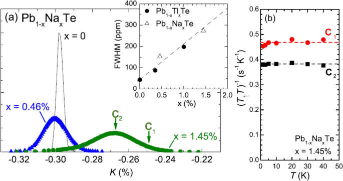
a ¹²⁵Te-NMR spectra in Pb _1−xNa_xTe at T = 20 K and B₀∼12 T for x = 0.46, and 1.45%. The inset shows the x dependence of the full width at half maximum (FWHM) of ¹²⁵Te-NMR spectra in Tl-doped and Na-doped PbTe compounds. b The 1/T₁T for x =1.45% are measured at the Te sites denoted by C_i (i = 1, 2) in the spectra of a

 Full size image 

Theoretically, it has been pointed out that the origin of enhancement in (1/T₁T) below ∼ 10 K is explained by the electron-pair hopping process between 6s electrons on the Tl dopants and the conduction electrons on the basis of the charge Kondo effect, as discussed in the next subsection.

Theoretical results for anomaly of NMR relaxation rate 1/T ₁

In this subsection, we discuss how the charge Kondo effect can give rise to the diverging behavior in the relaxation rate 1/T₁ across the Kondo temperature T_K, reinforcing that the charge Kondo effect is the origin of anomalous properties observed in Pb _1−xTl_xTe (0.006<x<0.015) [47].

An effective model Hamiltonian including the Coulomb interaction between the conduction electron and localized 6s orbital (denoted by d for manifesting the relation with the s-d model) is given by Eq. (22) in Section 3.1 with the hybridization between localized 6s orbital and conduction electrons:

\(\begin{array}{@{}rcl@{}} \mathcal{H}= \mathcal{H}_{\mathrm{c}}+\mathcal{H}_{\mathrm{d}} + \mathcal{H}_{\text{dc}} +\mathcal{H}_{\text{ph}} + \mathcal{H}_{\text{hyb}}, \end{array}\)

(56)

where

\(\begin{array}{@{}rcl@{}} \mathcal{H}_{\text{hyb}} &\equiv& V_{\text{dc}}\frac{1}{{\sqrt{N}}}\sum\limits_{\boldsymbol{k}\sigma} \left(c_{\boldsymbol{k}\sigma}^{\dagger}d_{\sigma}+\text{h.c.}\right), \end{array}\)

(57)

where N is the number of lattice sites. Hereafter, the origin of energy is taken as the Fermi energy of conduction electrons ε_F, the chemical potential at T=0, and the temperature T is assumed to be low enough compared to ε_F, i.e., T≪ε_F.

As discussed in Ref. [4], the pair-hopping interaction U_ph can stabilize the valence skipping state and cause the charge Kondo effect under certain condition. The origin of this phenomenon can be understood intuitively if we note that the U_ph is transformed to the pseudo-spin flipping exchange interaction (the origin of the Kondo effect) by the particle-hole transformation for the annihilation operators d_↓ and c_k↓.

The NMR relaxation rate 1/T₁ is given by the Moriya formula as [48]

\(\frac{1}{T_{1}T}=A^{2}\frac{1}{\omega}\text{Im} \Gamma^{\mathrm{R}}(\omega+\mathrm{i}\delta),\)

(58)

where A is the hyper-fine coupling constant between electron and nuclei, and Γ(iω_ν) is the transverse spin susceptibility of conduction electrons at certain Te site where NMR relaxation is observed and has several contributions, in general.

Considering the first order of U_ph, the total relaxation rate 1/T₁ is given by (See Ref. [47] for derivation)

\(\begin{array}{@{}rcl@{}} & &\frac{1}{T_{1}T}\approx A^{{2}} \frac{4\pi N_{\mathrm{F}}^{2}(V_{\text{dc}}N_{\mathrm{F}})^{2}} {\epsilon_{\mathrm{d}}^{2}}e^{-(r/\ell)} \left[\frac{\sin(k_{\mathrm{F}}r)}{k_{\mathrm{F}}r}J(k_{\mathrm{F}}r)\right]^{2}{T}\left[U_{\text{ph}}(T)-2U_{\text{dc}}(T)\right] \\ & &\qquad\quad +A^{2}\frac{12\pi N_{\mathrm{F}}^{2} (V_{\text{dc}}N_{\mathrm{F}})^{2}}{\epsilon_{\mathrm{d}}^{2}}e^{-(r/\ell)} \left[\frac{\text{sin}(k_{\mathrm{F}}r)}{k_{\mathrm{F}}r}J(k_{\mathrm{F}}r)\right]^{2}{T}U_{\text{dc}}(T), \end{array}\)

(59)

where r, l, and N_F are the distance between Tl impurity and the position of Te where 1/T₁T is measured, the mean-free path of conduction electrons, and the density of states of conduction band at the Fermi level, respectively. J(k_Fr) is an decaying and oscillating function of k_Fr like the Friedel oscillation function (see Fig. 2, Eqs. (21) and (22) in Ref. [47]). Since U_ph and U_dc correspond to J_⊥/2 and J_z/4 in the mapped world, respectively, the ratio of [U_ph(T)−2U_dc(T)] in the first term of Eq. (59) and U_ph(T) approaches zero toward T=T_K as decreasing temperature. Therefore, the first term gives less divergent behavior compared to the second term.

On the other hand, the second term in Eq. (59) exhibits pronounced increase as T decreases, toward T=T_K from the region \(T\gtrsim T_{\mathrm {K}}\), through the T dependence of TU_dc(T) (in a dimensionless form) shown in Fig. 14 in which the T dependence of U_dc(T) is given by the one-loop order RG (or poorman’s scaling) approximation as

\(U_{\text{dc}}(T)= \frac{1}{4N_{\mathrm{F}}\log\frac{T}{T_{\mathrm{K}}}}.\)

(60)

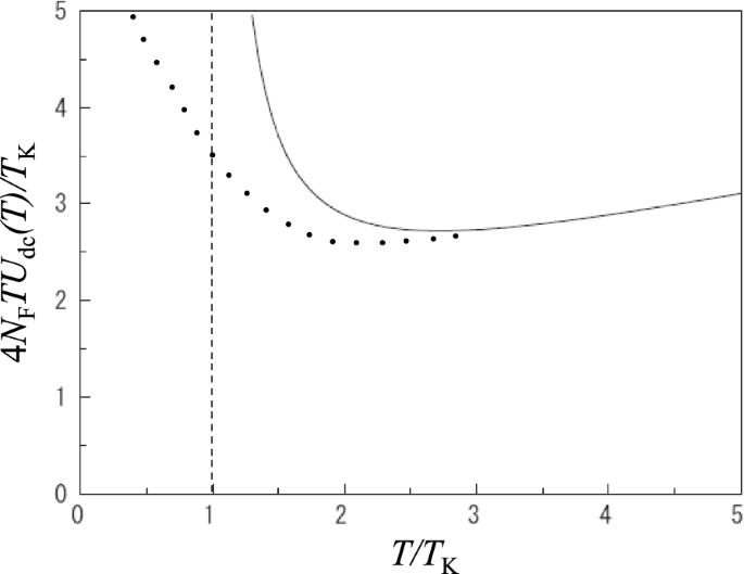
4N_FTU_dc(T)/T_K vs T/T_K with T_K being the Kondo temperature in the one-loop order RG (poorman’s scaling) approximation Eq. (60). Dotted line is a guide to the eyes for a qualitative behavior expected in exact treatment beyond poorman’s scaling solution as discussed in the text

 Full size image 

Of course, the result of poorman’s scaling ceases to be valid very near T=T_K. Nevertheless, it would give an increasing tendency of TU_dc(T) around T=T_K. The dotted line in Fig. 14 shows an expected T dependence of TU_dc(T) at T≲T_K, which is reasonable considering that the increasing tendency of TU_dc(T) already begins to appear at T≃2.7T_K, i.e., from far higher temperature than T_K, and that the divergent T dependence in U_dc(T) at T≪T_K works to suppress the Curie like divergence (∝1/T) of localized electron when entering into the local Fermi liquid state [49] in which the Kondo-Yosida charge singlet state is formed as in the case of magnetic Kondo problem [50].

Since the divergent part in (1/T₁T) Eq. (59) is in proportion to TU_dc(T), this theoretical result for (1/T₁T) qualitatively explains the anomalous temperature dependence of (1/T₁T) observed in Pb _1−xTl_xTe (x≃0.01) reported in Ref. [26]. However, of course to obtain more quantitative result for the T dependence in (1/T₁T) at T≲T_K, we need perform more solid calculations, such as numerical renormalization group method, which is left for future study.

Concluding this subsection, it is remarked that the present relaxation mechanism is quite different from the case of magnetic Kondo impurity in which (1/T₁T) is essentially in proportion to \(J_{\perp }^{2}\) as discussed in Ref. [51]. This difference is traced back to the difference in the order of perturbation process giving the relaxation rate. In the present case, (1/T₁T) is given by the first order process in the pair-hopping interaction U_ph and the inter-orbital interaction U_dc, while that in the case of magnetic Kondo impurity is given by the second order process in the s-d exchange interaction J_⊥ causing the spin-flip process, as discussed in Ref. [51]. In this scenario, the increase of Knight shift is also expected through the pair hopping interaction, which is consistent with the temperature dependence of Knight shift observed recently at dopant(Tl) site [47]. The experimental result of the Knight shift has been verified by explicit microscopic calculations similar to obtaining the anomalous behavior of the NMR relaxation rate 1/T₁, which will be published elsewhere.

There exists other possibilities of identifying superconductivity by valence skipping mechanism other than (Ba _1−xK_x)BiO₃ and Pb _1−xTl_xTe in which the valence skipping mechanism appears to play a crucial role. In this review, we briefly discuss the materials related with the valence skipping of Sn, In and Sb ions.

One of candidate materials on Sn ion is AgSnSe₂ which shows the superconductivity at T_c=4.5 K. The crystal structure of AgSnSe₂ is a face-centered cubic structure in which Ag and Sn are randomly occupied in the cation sites [52]. Since the band structure of SnSe, which is the face-centered cubic structure, is a nodal line semimetal [53], AgSnSe₂ is a heavily doped nodal line semimetal. By XAS and XPS measurements, the valence of Sn ion in AgSnSe₂ was reported to be Sn ²⁺ and Sn ⁴⁺, as the evidence of valence skipping state of Sn [54]. On the other hand, Sn-NMR spectra has suggested to be a Sn ³⁺ state which is the unusual valence state [55]. One of possible scenarios to understand this seemingly contradicting the usual valences of Sn ²⁺ and Sn ⁴⁺ is the difference of the time scale of probes. Namely, typical time scale of NMR measurement is far longer than that of e.g., the photo-emission spectroscopy so that the measured valence should be the average of degenerate valences Sn ²⁺ and Sn ⁴⁺. This unusual valence state of Sn ³⁺ has been recently reported also in SnP [56] and SnAs [57] where SnP and SnAs show a superconductivity at T_c∼3.4K (at P=0.45 GPa) and T_c∼3.58K. Although the experimental results on the valence state of Sn ion in AgSnSe₂ are still controversial, this material can be a good target material to understand the valence state of Sn ion in the material, and the relation between the origin of superconductivity and the valence of Sn ion. It should be noted that the valence state of Sn ion has been also discussed in NaSn₂As₂ which shows a superconductivity with T_c∼1.18K [58]. In addition, SnF₃, which is a candidate material utilizing the valence skip of Sn ion, has been predicted theoretically [59].

For In-doped Sn _1−δTe (Sn _1−x−δIn_xTe) which shows a superconductivity, the valence skipping of In ion has been discussed in [60]. This is because the carrier density does not change significantly as shown in Tl-doped PbTe [3], when In ions are doped.

The valence skipping effect and negative-U effect of Sb ion has been focused in (Ba,K)SbO₃ (BKSO) which is a similar material to BKBO, because BKSO shows a superconductivity with a maximum T_c of 15 K [61, 62].

In this paper, we reviewed historical researches and recent progress of valence skipping phenomena, especially focusing on the negative-U effect, the pair hopping interaction, suerconductivity, and the charge Kondo effect from both the theoretical and experimental sides.

The valence skipping is an unique phenomena especially in 5s and 6s states, while the valence skipping plays an important role as an origin of the exotic phenomenon such as a superconductivity and Kondo effect. Recently, there are many candidate materials related with the valence skipping as shown in Section 5, and thus, the another kinds of interesting phenomenon which are not superconductivity and charge Kondo effect will be expected. Indeed, one of the good examples is a thermoelectric effect: it is suggested that several materials with the valence skipper show a good thermoelectric performance by utilizing the lone pair effect, the impurity state due to the valence skipper, and so on. Therefore, the valence skipping phenomena have a potential of not only exotic phenomenon but also an application to the materials which are important to the realization of the sustainable society.