Introduction
The geometric and topological methods provide new insights to quantum systems in condensed matter physics [1,2,3,4]. It has been found that the quantum Hall and spin Hall effects can be understood in terms of the topological states identified by the Chern classes, \(\mathbb {Z}\) and \(\mathbb {Z}_{2}\) [5,6,7,8]. These discoveries have attracted many attempts to explore the topological phases in condensed matter systems based on the symmetry group and homological invariants [7, 8]. The concepts of the Berry connection and curvature in quantum systems provide a geometric approach to understand quantum states and their evolutions [9, 10]. The winding number and Chern number are identified the topological phases and their phase transitions [4]. Recently, these concepts ware generalized to non-Hermitian quantum systems and its holonomy interpretation [11,12,13,14]. One found that the complex energy band structures of non-Hermitian systems show rich physics beyond Hermitian systems. Especially the complex band gaps and their corresponding exceptional points associate with topological phases [13]. The complex Berry phase for non-Hermitian systems has been proposed and applied to study the behaviors near the exceptional point [15,16,17], dissipative behaviors [18, 19], and quantum phase transition [20, 21]. In particular, the Berry phase are generalized to the global Berry phase, which play a role of the winding number to identify the topological invariants in the non-Hermitian quantum walk and dissipative bipartite lattice [21,22,23]. The robust topological states promise potential applications in quantum materials and technologies [24,25,26].
Quantum non-Hermitian systems exhibit unconventional characteristics and potential applications [11, 24, 27,28,29,30]. In particular, non-Hermiticity of systems describes some dissipative phenomena, such as energy gain or loss and non-conserved probability of electrons appearing [31,32,33]. These unconventional characteristics beyond standard quantum mechanics yield many novel phenomena in quantum states, such as the 10-fold topological equivalent classes in Hermitian systems based on the Altland-Zirnbauer (AZ) symmetry classification are extended to the 38-fold topological equivalent classes due to the additional sublattice symmetry and pseudo-Hermticity in non-Hermitian systems [12, 13]. One found that the complex energy band gap could form a point or line gap to preserves its topological invariants under a unitary or Hermitian flattening transformation [13]. The energy band gaps close to form the exceptional points and lines as the reference points or lines associated with the topological phases [12, 13]. Moreover, the non-Hermiticity of systems deforms the Bloch-wave behavior to yield the skin effect for lattice models [34,35,36,37]. One introduced the biorthogonal polarization to modify the conventional bulk-boundary correspondence to show the zero modes [38,39,40], the topological edge states, and the finite-size effects in the non-Hermitian Su-Schrieffer-Heeger (SSH) model [41,42,43,44,45]. In particular, Chen and Zhai studied the Hall conductance of a non-Hermitian Chern insulator and found some deviations of the quantized Chern number and the quantum Hall conductance [44,45,46].
In particular, one found that all eigen energies of the non-Hermitian systems are still real if the systems have \(\mathcal{PT}\mathcal{}\) (Parity-Time reversal) symmetries or pseudo-Hermitian symmetry [31, 32]. The quantum evolution driven by non-Hermitian Hamiltonian with the \(\mathcal{PT}\mathcal{}\) symmetry is faster than those driven by Hermitian Hamiltonian [47, 48], which provides a novel insight to quantum computation. Moreover, the time reversal symmetry and its relevant topological invariants have been studied extensively and applied in electromagnetism, compact star matter and quantum computation [49,50,51,52,53].
More interestingly, the quantum Hall conductance in the Dirac model can be generalized to quantum Hall admittance in the non-Hermitian Dirac model. Namely the quantum Hall susceptance emerges, such as quantum Hall capacity and induction [54]. This inspires fundamental insights into non-Hermitian systems and lead to potential applications [54]. One found that the edge states in the complex energy band play an important role in the topological invariants and the topological phase transition in the non-Hermitian systems [55]. These topological invariants are associated with the velocity field of the Bloch electrons in the Brillouin zone and connected to the Euler index [56].
On the other hand, as a typical two-dimensional (2D) system, graphene promises great potential applications in nanoelectronics and nanotechnology [57, 58]. Its honeycomb lattice structure yields the Dirac cone in its energy band structure. Graphene provides a practical system to explore the geometric and topological properties of the Dirac model in condensed matter systems [59]. However, most of the previous theoretical works focus on the Hermitian graphene model [59,60,61]. When we consider that the graphene is on a substrate in some practical applications, there should be exist coupling between the graphene and the substrate, which may induce the dissipative effect due to asymmetric carbons in the hexagon lattice. Thus, these dissipative effects in the graphene may be modeled by a non-Hermitian graphene model.
In this paper, we study the geometric and topological features of the non-Hermitian graphene model. Firstly, we propose a non-Hermitian Hamiltonian of graphene based on the tight-binding approximation in the Section 2. The dissipative effects come from the coupling of the graphene with the substrate. In Section 3, we analyze the symmetry of this model and its relationship with the exceptional point and topological invariants. In Sections 4 and 5, we give analytically the complex Berry connection and the complex Berry curvature of this non-Hermitian graphene model. Then in Section 6, we investigate numerically the relationship between the complex Berry curvature and the complex energy band structure. Finally, we give the conclusions and outlook in Section 7.
Non-Hermitian graphene model
Let us consider a honeycomb lattice, where there are two kinds of atoms, A and B shown in Fig. 1. The graphene can be modeled by the tight-binding approach with the equal on-site energies of A and B atoms. When the graphene couples the substrate, in which A and B atoms will gain or loss energy asymmetrically such that graphene becomes a dissipative system. This dissipative mechanism can be modeled by a non-Hermitian graphene model. Its Hamiltonian can be expressed as [57, 58]
where \(\epsilon _A\) is the on-site energy of A sites, while \(\epsilon _B=\epsilon _A-i2\Gamma\) is the on-site energy of B sites, and the imaginary part describes the dissipation. When \(\Gamma =0\), the Hamiltonian H reduces to the Hermitian graphene Hamiltonian. Using Fourier transformation, we can rewrite the Hamiltonian in the reciprocal space,
where \(\Psi ^\dagger _\mathbf {k}=\left( a_\mathbf {k}^\dagger , b_\mathbf {k}^\dagger \right)\) and
is the Hamiltonian in the reciprocal space with
with a being the lattice constant of the graphene. We set \(\hbar =1\) and \(a=1\) for convenience in the following sections. By solving the eigenequation, we can obtain the eigenvalues
where \(\eta =\frac{\Gamma }{t}\). The corresponding eigenvectors are
and their dual eigenvectors in the dual space are
where cos and sin are complex functions and * means the complex conjugated operator. We define
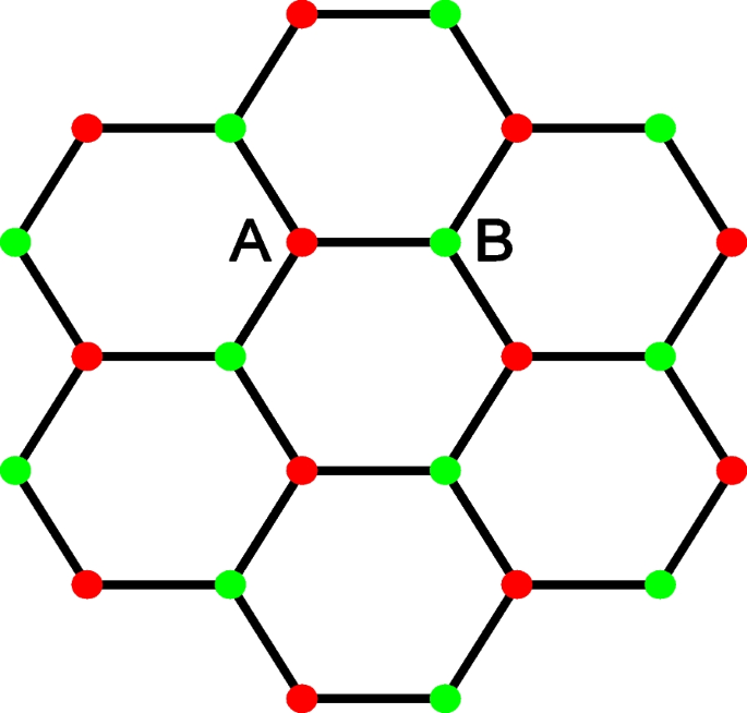
(Color online): The honeycomb lattice, where A and B label two different sites of the graphene
It should be pointed out that studying the non-Hermitian graphene model will turn out the two-fold physical meanings. (1) Graphene shows many interesting properties and potential applications due to its hexagonal lattice structure. When we design a quantum device based on the graphene, the A and B atoms in graphene couple asymmetrically to substrate which gain or lose different energy such that the graphene becomes a non-Hermitian systems. To understand this non-Hermitian graphene model will help us to further design quantum devices based on the graphene with the dissipative phenomena [57, 58]. (2) The non-Hermitian graphene model can be reduced to the non-Hermitian Dirac model in the low energy domain, which involves many fundamental issues, such as the geometric properties and topological invariants of quantum states. Actually, the non-Hermiticity of quantum systems has attracted many attempts to understand symmetry and topological invariants [13, 62].
Symmetries, exceptional points, and topological invariants
In general, all energy bands are real for Hermitian systems such that the energy band gap near Fermi energy can be regarded topologically as a point called point gap. However, for the non-Hermitian systems, the energy bands could be complex such that the energy band gaps can be classified topologically to either point or line gaps in the complex energy plane. When the energy band gap closes, the topological phase transition between the trivial and topological phases [13, 62].
Note that the diagonal elements of \(h_\mathbf {k}\) are neither equal nor complex conjugated, we have
where \(\mathcal {P}\) is the parity operator and \(\mathcal {T}\) is the time reversal operator. \(\xi\) is a unitary and Hermitian matrix [13, 32]. In other words, both \(\mathcal{PT}\mathcal{}\) and pseudo-Hermitian symmetries do not hold for this non-Hermitian graphene model. However, with the parameters varying, the occurrence of the exceptional points (gapless modes) at some \(\mathbf {k}\) points in the Brillouin zone may lead to the topological phase transition.
Let us examine the exceptional points of the energy band structure in the Brillouin zone and their corresponding parameters, the energy band (5) gives that the gapless modes satisfy equation \(\mid f_\mathbf {k}\mid ^2-\eta ^2=0\), which yields
In particular, for \(\eta =1\), \(\cos \frac{\sqrt{3}k_y}{2}=0\) infers \(k_y=\pm \frac{\pi }{\sqrt{3}}\) with \(0\le k_x\le 2\pi\), or \(\cos \frac{\sqrt{3}k_y}{2}+\cos \frac{3k_x}{2}=0\) yields
which implies that the line gap may occur along these two lines in the Brillouin zone, which could be mapped to the complex energy plane. On the other hand, by maximizing and minimizing cosine functions in (10), the range of \(\eta\) for the exceptional points (gapless) is obtained as \(1\le \eta \le 3\).
It should be remarked that the occurrence of the exceptional point implies the existence of the topological phase for non-Hermitian systems even though the system does not contain the \(\mathcal{PT}\mathcal{}\) and pseudo-Hermitian symmetries. In particular, the occurrence of the exceptional point is associated with the divergence of the Berry curvature. We will see this connection in the Section 6. Usually, the winding number or vorticity can be identified the exceptional point appearing inside or outside of the integral loop even for non-Hermitian systems [62]. How to connect the topological invariants of the quantum states to the physical observables and phenomena is worth studying further.
Berry connection and complex Berry phase
The Berry connection can be generalized to \(A_{\alpha \beta }:=i\langle \widetilde{\psi }_{\alpha }|d|\psi _{\beta }\rangle\) for non-Hermitian systems. The matrix form is expressed as [21]
Using the eigenvectors in (6) and (7), the Berry connection can be obtained by
where \(\sigma _0=\mathbf {1}_{2\times 2}\) is the identity matrix, and \(\sigma _{x,y,z}\) are Pauli’s matrices. The sine and cosine functions are defined by (see (8a)),
The Berry phase is defined by \(\gamma _{\pm }=\oint _{C}A_{\pm }\), where \(A_{\pm }\) are the diagonal elements in (12), respectively. The loop integral means that the Berry phase depends on the cyclic quantum evolution in the parameter (or \(\mathbf {k}\)) space. Using (12), we can obtain the Berry phase,
which is in general complex because the Hamiltonian is non-Hermitian. Using (8b), we have \(d\theta _k=\nabla _{\mathbf {k}}\arg (f_\mathbf {k})\cdot d\mathbf {k}\), and the Berry phase can be expressed as
Note that
then we obtain
Complex Berry curvature
The Berry curvature defined by \(F=dA\) plays a gauge field for the Hermitian system. For the non-Hermitian system, the Berry connection is generalized to complex domain such that the Berry curvature is also generalized to complex domain. In order to give the explicit expression of the complex Berry curvature, the Berry connection in Eq. (12) can be rewritten as
where
Using (8a), we have
We obtain the coordinate transformation from the \((\theta _{k},\phi )\)-space to the \((k_{x},k_{y})\)-space.
Thus, the Berry connection in Eq. (18) can be expressed in terms of k space
where
with
The z-component of Berry curvature is defined by the 2-form
The partial derivative of (24) is given by
Note that \(\frac{\partial P_\mathbf {k} }{\partial k_{x}}\frac{\partial \mid f_\mathbf {k}\mid }{\partial k_{y}}-\frac{\partial P_\mathbf {k} }{\partial k_{y}}\frac{\partial \mid f_\mathbf {k}\mid }{\partial k_{x}}=0\) and
with (21), we get
By substituting above equations to Eq.(27), we finally obtain the 2-form Berry curvature.
where \(\mathcal {F}_z=\left( \alpha _{\mathbf {k}}\sigma _{x}+\beta _{\mathbf {k}}\sigma _{z}\right)\) with
where
then
The complex 2-form Berry curvature can be rewritten to the real and imaginary parts,
For \(\mid f_\mathbf {k}\mid ^{2}-\eta ^{2}>0\),
For \(\mid f_\mathbf {k}\mid ^{2}-\eta ^{2}<0\),
It should be remarked that the non-Hermiticity \(\eta\) of the system induces the Berry curvature. When \(\eta \rightarrow 0\), \(\mathcal {F}_z\rightarrow 0\) which may be called the Berry flat. The Berry curvature can be regarded as a 2-form non-Abelian gauge field. Its components are represented a \(2\times 2\)-matrix. The real and complex components are related to the Pauli’s matrix \(\sigma _x\) and \(\sigma _z\) in (35) and (36).
Relationships between complex Berry curvature and complex energy band structure
In order to reveal the physical mechanism of the complex Berry curvature, We analyze the relationship between the complex Berry curvature and the energy band structure of the non-Hermitian graphene model. It can be seen that \(\mathcal {F}_z\) is in general complex. At some points \(\mid f_\mathbf {k}\mid =\eta\) in the Brillouin zone for given \(\eta\), the real and imaginary parts of the curvature \(\mathcal {F}_z^r\) and \(\mathcal {F}_z^i\) diverge, which corresponds to the energy gap closing (see Eq. (5)).
We plot numerically the complex energy bands in the Brillouin zone in Fig. 2, where we set \(\epsilon _A=0\) without lose of generality. It can be seen that the energy band structures show quite different structures with the non-Hermitian parameter \(\eta\). The real and imaginary parts of the valence and conduction bands, \(\mathrm {Re}(E_{\pm })\) and \(\mathrm {Im}(E_{\pm })\), are symmetric and depend on the non-Hermitian parameter \(\eta\). They show three typical structures in the parameter space.
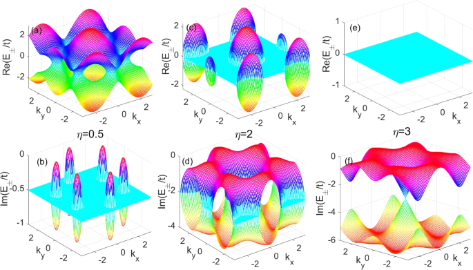
(Color online): The complex energy band structures in Brillouin zone for different parameter parameters \(\eta\). a, b The real and imaginary parts of the complex energy structure in \(\eta =0.5\). c, d The real and imaginary parts of the complex energy structure in \(\eta =2\). e, f The real and imaginary parts of the complex energy structure in \(\eta =3\). We set \(\epsilon _A=0\)
For the parameter \(\eta =0.5\), both of \(\mathrm {Re}(E_{\pm })\) and \(\mathrm {Im}(E_{\pm })\) of the energy bands show some cave structures in the Brillouin zone and the gaps of \(\mathrm {Re}(E_{\pm })\) and \(\mathrm {Im}(E_{\pm })\) close in some k regions. There is a big cave of \(\mathrm {Re}(E_{\pm })\) in the center (\(\Gamma\) point) of the Brillouin zone and six-half caves of \(\mathrm {Re}(E_{\pm })\) located at the corner (K,K’ points) of the Brillouin zone. For the imaginary part of the energy band, \(\mathrm {Im}(E_{\pm })\), there are six small caves appearing at the corners of the Brillouin zone. It should be noted that the caves of \(\mathrm {Re}(E_{\pm })\) are connected, but the caves of \(\mathrm {Im}(E_{\pm })\) are separated by the flat regions in the Brillouin zone (see in Fig. 2a and b). As \(\eta\) increases and reach 2, the caves of the \(\mathrm {Re}(E_{\pm })\) become separated and the caves of \(\mathrm {Im}(E_{\pm })\) become connected at \(\eta =2\) shown in Fig. 2 c and d.
When the parameter \(\eta\) increases further, the real part of the energy band \(\mathrm {Re}(E_{\pm })\) continuously deformed into a smaller disk and finally vanish in the Brilouin zone for \(\eta =3\) shown in Fig. 2 e and f. The imaginary part of the energy band \(\mathrm {Im}(E_{\pm })\) forms a Dirac-like cone at the \(\Gamma\) point in the Brillouin zone. When the parameter increases further \(\eta \ge 3\), \(\mathrm {Re}(E_{\pm })=0\), but the gap of \(\mathrm {Im}(E_{\pm })\) emerges at the \(\Gamma\) point of Brillouin zone [63]. What physical phenomena observed from this complex energy structure are worth studying further.
In general, the complex energy gap closing with the parameter varying in the non-Hermitian systems occurs at the exceptional degeneracy associated with the topological phase depending on the symmetry of systems, such as the topological phase characterized by the Chern number for quantum Hall systems or winding number for Su-Schrieffer-Heeger model [13, 34].
In Figs. 3, 4, and 5, we plot the diagonal and off-diagonal components of the complex Berry curvature matrix with several non-Hermitian parameters \(\eta\) in the Brillouin zone. For \(\eta =0.5\) shown in Fig. 3 from a to d, we can see that there are several small peaks of the curvature components \(\mathrm {Re}(\mathcal {F}_{11}), \mathrm {Im}(\mathcal {F}_{11})\), \(\mathrm {Re}(\mathcal {F}_{12})\), and \(\mathrm {Im}(\mathcal {F}_{12})\) appearing in the Brillouin zone. The peaks for the \(\mathrm {Re}(\mathcal {F}_{11})\) and \(\mathrm {Im}(\mathcal {F}_{12})\) are much higher than those of the \(\mathrm {Im}(\mathcal {F}_{11})\) and \(\mathrm {Re}(\mathcal {F}_{12})\). As the parameter increases to \(\eta =2\) in Fig. 4 from a to d, the peaks of the complex components of the curvatures become sharp and high. When the parameter increases further to \(\eta =3\) in Fig. 5 from a to d, all peaks of the complex curvatures return to be fat and low.
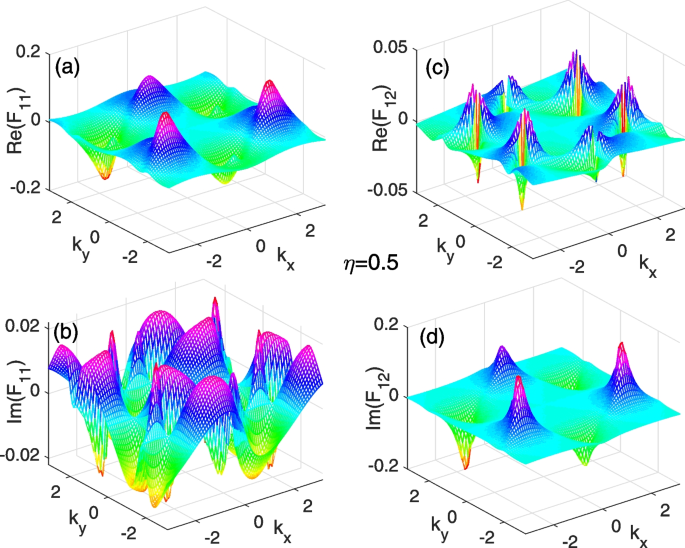
(Color online): The complex Berry curvatures in the Brillouin zone for the parameter parameters \(\eta =0.5\). a and b are the real and imaginary parts of the diagonal component of the complex Berry curvature \(\mathcal{F}_{11}\), respectively. c and d are the real and imaginary parts of the off-diagonal complex Berry curvature \(\mathcal{F}_{12}\), respectively
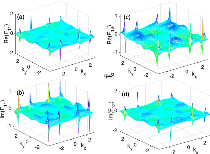
(Color online): The complex Berry curvatures in the Brillouin zone for the parameter parameters \(\eta =2\). a and b are the real and imaginary parts of the diagonal component of the complex Berry curvature \(\mathcal{F}_{11}\), respectively. c and d are the real and imaginary parts of the off-diagonal complex Berry curvature \(\mathcal{F}_{12}\) , respectively
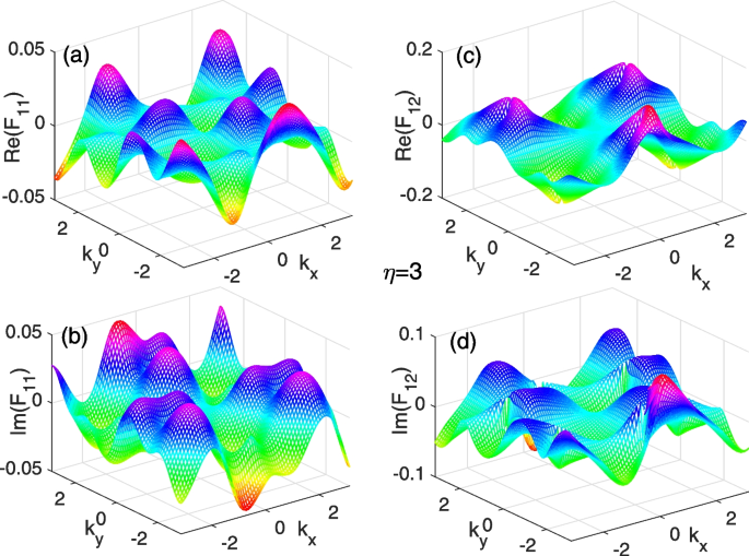
(Color online): The complex Berry curvatures in the Brillouin zone for the parameter parameters \(\eta =3\). a and b are the real and imaginary parts of the diagonal component of the complex Berry curvature \(\mathcal{F}_{11}\), respectively. c and d are the real and imaginary parts of the off-diagonal complex Berry curvature \(\mathcal{F}_{12}\), respectively
In general, the behaviors of the complex curvature depend on the energy band structure. The peaks of the complex curvatures appear at the exceptional (gapless) points \(\mid f_\mathbf {k}\mid ^2\rightarrow \eta ^2\) in the Brillouin zone for given \(\eta\). The peak appearance should be associated with some physical phenomena. This is still an open question for further study.
In principle, the non-Hermitian part of the Hamiltonian describes some dissipative or non-conserved phenomena of systems. It can be seen that the Berry curvature plays a non-Abelian gauge field. The Berry gauge field is observable. The Berry curvature \(\mathcal {F}\) divergence may provide a measurable signal to detect the quantum phase transition in non-Hermitian systems.
Conclusions and outlook
Graphene as a typical 2D material has been attracted a lot of efforts for potential applications in nanoelectronics and many attempts to explore the fundamental issues, such as the quantum Hall conductance in the graphene system, which is expressed in terms of the Chern number [64, 65]. In particular, non-Hermitian quantum systems describe dissipative phenomena, which exhibit rich physics beyond Hermitian systems due to their complex energy band structures [13, 33].
In this paper, we have considered the non-Hermitian graphene model to describe the asymmetric coupling between the graphene and the substrate based on the tight-binding approximation. We have given analytically the complex Berry connection and Berry curvature of this non-Hermitian graphene model and numerically investigated the relationship between the complex Berry curvature and the complex energy structure. The behaviors of the complex Berry curvature depend on the complex energy band structure and the non-Hermitian parameter \(\eta\). In particular, we find that some cave structures of both real and imaginary parts of the energy bands occur in the Brillouin zone. Interestingly, the Dirac cone of the imaginary energy band emerges and the flat structure of the real part of the energy band for \(\eta =3\). These imply some hints for the topological invariants in the non-Hermitian graphene. The complex Berry curvature and its non-analytic behaviors in the Brillouin zone provides a way to explore quantum phase transition [15, 20,21,22]. The occurence of the peaks of the Berry curvature corresponds to the exceptional (gapless) points. Actually, there are still some puzzles for studying further. For example, whether the non-analytic behaviors of the complex Berry curvature are related to the topological invariants like quantum Hall conductance and admittance [54].
From the mathematical point of views, the complex curvature may be related to complex geometry and complex manifold. These open a connection between theoretical physics and mathematics [66]. In particular, the occurence of the Dirac cone of the energy bands involves the Dirac equation, which implies the relativistic effect or the Minkowski geometry appearing in condensed matter systems. These results provide a novel insight to the relationship between the non-Hermitian quantum, geometry, and topological invariants as well as their applications.