Abstract
Inspired by the astonishing \(7\sigma\) discrepancy between the recent CDF-II measurement and the standard model prediction on the mass of W-boson, we investigate the \(\lambda '\)-corrections to the vertex of \(\mu \rightarrow \nu _\mu e\bar{\nu _e}\) decay in the context of the R-parity violating minimal supersymmetric standard model. These corrections can raise the W-boson mass independently. Combined with recent Z-pole and kaon decay measurements, \(m_W \lesssim 80.37\) GeV can be reached. We find that these vertex corrections cannot explain the CDF result entirely at the \(2\sigma\) and even \(3\sigma\) levels. However, these corrections together with the oblique contributions can be accordant with the CDF-II result and relevant bounds at the \(3\sigma\) level.
1 Introduction
In the past decades, the observation of striking agreement between the standard model (SM) predictions and the experimental results in a vast number of particle interactions has shown up the powerful predicted capacity of the SM. However, the SM is not the final answer to the particle physics, as it is unable to explain several phenomena, including the matter-antimatter asymmetry, the origin of neutrino mass, the hierarchy problem, and the candidate of dark matter. These strongly call for some new physics (NP) beyond the SM. Although no up-to-date direct evidence shows that the NP exists, there are still indirect ways, e.g., studying the loop-effects of NP on low-energy processes or electroweak observables, like the precision measurement of the W-boson mass.
Recently, the Collider Detector at Fermilab (CDF) collaboration at Tevatron reported a high precision measurement on the mass of W-boson with the CDF-II detector. The measured value is given by \(m_W^{\text {CDF}}=80.4335\pm 0.0094~\text {GeV}\) [1] with better precision than all other previous measurements and is \(7\sigma\) from the SM prediction \(m_W^\text {SM}=80.357\pm 0.006~\text {GeV}\) [2]. If the measurement is confirmed in the future, such an astonishing tension will undoubtedly be a strong challenge to the SM. After this exciting \(m_W^\text {CDF}\) reported, plentiful theoretical researches [3,4,5,6,7,8,9,10,11,12,13,14,15,16,17,18,19,20,21,22,23,24,25,26,27,28,29,30,31,32,33,34,35,36,37,38] have emerged in a short time.
Before this profound result, there are already some anomalies indicating the clues of NP, e.g., the recent average values of the observables \(R_{D^{(*)}}\), reported by the Heavy Flavor Averaging Group [39,40,41], are about \(3.2\sigma\) away from the corresponding SM predictions [42,43,44,45,46,47,48,49,50], considering the \(R_{D}\) and \(R_{D^*}\) total correlation \(-0.29\). To explain these anomalies, there are numerous phenomenological studies combined with the \(m_W^{\text {CDF}}\) measurement in different models (e.g., see Refs. [34, 51,52,53,54,55]). In this work, we utilize the minimal supersymmetric standard model (MSSM) extended by the R-parity violation (RPV), especially including the \(\lambda '\hat{L} \hat{Q} \hat{D}\) superpotential term, which can explain the B-physics anomalies in the neutral currentFootnote 1 or/and the charged one (see, e.g., Refs. [62,63,64,65]). Thus, further investigations on this framework for the \(m_W^{\text {CDF}}\) explanation are necessary. Although it is found that the MSSM can provide some parameter points which can raise \(m_W\) into the \(2\sigma\) accordance region [9], mainly through bosonic self-energy contributions relevant to the oblique corrections [66, 67], the stop mass in the solution with \(m_{\tilde{t}}\lesssim 1\) TeV is not suit for general collider search scenarios. Thus, it is also worth studying other corrections to \(m_W\) in the extended MSSM framework, considering the general bounds for colored sparticle masses at the Large Hadron Collider (LHC). Above all, we will study corrections to the vertex \(W\ell \nu\) from the R-parity violating interaction \(\lambda '\hat{L} \hat{Q} \hat{D}\) and get an enhancement to \(m_W\), which is independent of the oblique corrections.
This paper is organized as follows. In Section 2, we introduce the vertex corrections to the W-boson mass in the MSSM framework extended by RPV. Then, we show the numerical results and discussions in Section 3. Our conclusions are presented in Section 4.
2 The contribution to \(m_W\) from the R-parity violating MSSM
As we know, the W-boson mass can be determined from the muon decay with the relation (see, e.g., Refs. [68,69,70])
which comprises the three precise inputs, the Z-boson mass \(m_Z\), the Fermi constant \(G_\mu\), and the fine structure constant \(\alpha\). Here the one-loop corrections to \(\Delta r\) can be expressed as
where the SM part \(\Delta r^{\text {SM}}\) is derived first in Refs. [71, 72]. Within the NP part, the self-energy of the renormalized W-boson is denoted by \(h^s\), and the vertex and box corrections to the \(\mu \rightarrow \nu _\mu e\bar{\nu _e}\) decay are denoted by \(h^v\) and \(h^b\), respectively. In the MSSM, the pure squarks (sleptons) only engage the self-energy sector at the one-loop level. The corrections to the vertex and box involve charginos and neutralinos. Among these one-loop contributions in the MSSM, the dominant contribution to \(m_W\) is the one-loop diagrams involving pure squarks. This dominant part in \(h^s\) can be expressed by [68]
where \(\theta _W\) is the Weinberg angle and the definition of mixing angle \(\theta _{\tilde{q}}\) is referred to Ref. [68] and the function \(F_0(x,y)=x+y-\frac{2xy}{x-y} \log \frac{x}{y}\) with the extra properties \(F_0(m^2,m^2)=0\) and \(F_0(m^2,0)=m^2\). Thus, one can see that \(h^s\) is sensitive to the mass splitting between the isospin partners due to the factor \(\cos ^2 \theta _{\tilde{t}} \cos ^2 \theta _{\tilde{b}}\). Obviously, \(h^s\) can be negligible when the soft breaking masses \(M_{\tilde{Q}_i}\) are sufficiently heavy compared to the chiral mixing. In this work, we focus on the vertex corrections \(h^v\) affected by the \(\lambda '\)-coupling in the R-parity violating MSSM (RPV-MSSM) and can omit \(h^s\) and \(h^b\) in the particular scenario.
In RPV-MSSM, the \(\lambda '\)-superpotential term \(\mathcal{W}=\lambda '_{ijk} \hat{L}_i \hat{Q}_j \hat{D}_k\) leads to the related Lagrangian in the mass basis
where the generation indices \(i,j,k=1,2,3\), while the color ones are omitted, and “c” indicates the charge conjugated fermions. In this paper, all the repeated indices are defaulted to be summed over unless otherwise stated. The relation between \(\lambda '\) and \(\tilde{\lambda }'\) is \(\tilde{\lambda }'_{ijk}=\lambda '_{ij'k} K^{*}_{jj'}\) with K being the Cabibbo-Kobayashi-Maskawa (CKM) matrix. In this work, we restrict the index k of the superfield \(\hat{D}_k\) to the single value 3.
Including the one-loop contribution from the RPV-MSSM, the \(W \ell _l \nu _{i}\)-vertex is described by the following Lagrangian
where g is the \({\text {SU}}(2)_L\) gauge coupling, and the correction part \(h_{li}\) from the \(\lambda '\)-contributions is given by (as the analogy to the formula in Ref. [73])
where \(x_t \equiv m^2_t/m^2_{\tilde{b}_R}\) and the loop function \(f_W(x) \equiv \frac{1}{x-1} + \frac{(x-2) \log x}{(x-1)^2}\) and other non-dominant parts are eliminated. This dominant contribution is from the vertex engaged by the right-handed sbottom \(\tilde{b}_R\) (Fig. 1a) while the vertex involving left-handed squarks (Fig. 1b) provides non-dominant effects and can be eliminated. Then, we consider the \(\lambda '\)-correction only to the \(W\mu \nu\)-vertex or to the \(We\nu\)-vertex at a time. This can be easily achieved by setting one of the couplings \((\tilde{\lambda }'_{133}, \tilde{\lambda }'_{233})\) dominant while neglecting the rest. Given this “single coefficient dominance” scenario, the \(\lambda '\)-corrections to the \(\mu \rightarrow \nu _\mu e\bar{\nu _e}\) box also vanish,Footnote 2 then the one-loop \(\lambda '\)-contribution to \(\Delta r\) only comes from \(h'_{aa}\) (the index a here is restricted to 1 or 2 at a time).
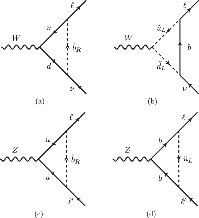
The diagrams of the \(W\ell \nu\)-vertex and \(Z\ell \ell ^{(')}\)-vertex (shown as examples) in the RPV-MSSM
Given the purpose of this work is to investigate that to what degree, the pure \(\lambda '\) contribution, \(h'_{aa}\), can accommodate the new W-boson mass data. We can further write down the prediction of the W-boson from the pure-\(\lambda '\) contributionsFootnote 3 as
with Eqs. (1) and (6). It is clear from Eq. (7) that the right-handed sbottom mass \(m_{\tilde{b}_R}\) and the coupling \(\tilde{\lambda }'_{a33}\) are related to \(\lambda '\)-correction of \(m_W\).
3 Numerical results and discussions
In this section, we investigate the explanation of \(m_W^{\text {CDF}}\) combined with the relevant constraints. At first, we concentrate on the pure \(\lambda '\)-effects assuming the soft breaking masses of gauginos and left-handed squarks (sleptons) are sufficiently heavy, and then, only the model parameters \((\tilde{\lambda }'_{a33},m_{\tilde{b}_R})\) are involved. If the pure \(\lambda '\)-contribution (see Eq. (7)) can explain the new W-boson mass at the \(2\sigma\) level, we need \(h'_{aa}\) to fulfill \(-6.34
Also, \(-6.34
stay in the region
because \(R^W_{\text {NP/SM}}\) can be calculated as \(1+2h'_{aa}\), with Eq. (5). Then, we compare Eq. (10) with the W-boson partial width ratios \(R^W_{l/l'}\equiv \Gamma (W\rightarrow l\nu )/\Gamma (W\rightarrow l'\nu )\), and their experimental results are given as \(R^W_{\mu /e}=0.996\pm 0.008\), \(R^W_{\tau /\mu }=1.008\pm 0.031\), and \(R^W_{\tau /e}=1.043\pm 0.024\) [74]. It is found that the \(m_W\) explanation demands much stronger bounds, whenever the NP exists in the \(\mu\) or e channel (the \(\tau\) flavor is assumed decoupled with the NP for simplicity).
As shown in Fig. 1c and d, the NP effects on the \(W\ell \nu\)-vertex will also inevitably affect the Z-vertex. The Z-boson partial width ratios \(R^Z_{l/l'}\equiv \Gamma (Z\rightarrow ll)/\Gamma (Z\rightarrow l'l')\) are measured as \(R^Z_{\mu /e}=1.0001\pm 0.0024\), \(R^Z_{\tau /\mu }=1.0010\pm 0.0026\), and \(R^Z_{\tau /e}=1.0020\pm 0.0032\) [74], which all constrain the coupling \(g_{\ell _L}\) in the effective Lagrangian
where \(g_{\ell _L}^{ij}=\delta ^{ij}g_{\ell _L}^{\text {SM}}+\delta g_{\ell _L}^{ij}+\delta g_{\ell _L}^{\prime ij}\) and \(g_{\ell _R}^{ij}=\delta ^{ij}g_{\ell _R}^{\text {SM}}\), with \(g_{\ell _L}^{\text {SM}}=-\frac{1}{2}+\sin ^2\theta _W\) and \(g_{\ell _R}^{\text {SM}}=\sin ^2\theta _W\). The formulas of \(\delta g_{\ell _L}^{ij}\) and \(\delta g_{\ell _L}^{\prime ij}\) are [75]
Here we can define \(B^{ij} \equiv (32\pi ^2) (\delta g_{\ell _L}^{ij}+\delta g_{\ell _L}^{\prime ij})\) and further get the bound \(|B^{aa}|<0.35(0.53)\) at the \(2(3)\sigma\) level. Given that the mass of \(\tilde{t}_L\) is set sufficiently heavy, the \(\delta g_{\ell _L}^{\prime ij}\) part can be eliminated.
As to the invisible Z-decay, this model can also make loop-level contributions to the \(Z\rightarrow \nu \bar{\nu }\), i.e., \(\ell\) exchanged with \(\nu\) and u(\(\tilde{u}_L\)) exchanged by d(\(\tilde{d}_L\)) in Fig. 1c, d. Then, the effective number of light neutrinos \(N_\nu\), which is defined by \(\Gamma _{\text {inv}}=N_\nu \Gamma _{\nu \bar{\nu }}^{\text {SM}}\) [76], will constrain the couplings via
where the coupling \(\delta g_{\nu }^{\text {SM}}=\frac{1}{2}\) and the formulas of \(\delta g_{\nu }^{(\prime )ij}\) is given by
Then, the measurement \(N_\nu ^{\text {exp}}=2.9840(82)\) [76] will make constraints.
Except the purely leptonic decays of W/Z boson, the \(\mu \rightarrow e\bar{\nu }_e\nu _\mu\) and \(\tau \rightarrow \ell \bar{\nu }_{\ell }\nu _\tau\) decays, which contain the \(W\ell \nu\)-vertex, should also be considered. The fraction ratios \(\mathcal{B}(\tau \rightarrow \mu \bar{\nu }_\mu \nu _\tau )/\mathcal{B}(\tau \rightarrow e\bar{\nu }_e\nu _\tau )\), \(\mathcal{B}(\tau \rightarrow e\bar{\nu }_e\nu _\tau )/\mathcal{B}(\mu \rightarrow e\bar{\nu }_e\nu _\mu )\), and \(\mathcal{B}(\tau \rightarrow \mu \bar{\nu }_\mu \nu _\tau )/\mathcal{B}(\mu \rightarrow e\bar{\nu }_e\nu _\mu )\) make the bounds [77] as
Due to that \(h'_{aa}\leqslant 0\), Eq. (15) induces the \(2(3)\sigma\) bounds \(-4.6(-6.0)
Combining the bounds introduced above with the W mass explanation, the allowed regions are shown in Fig. 2. The two areas allowed by \(Z\rightarrow \ell \ell\) and kaon decays overlap almost entirely at the \(2\sigma\) level, while the \(Z\rightarrow \ell \ell\) bound is stronger at the \(3\sigma\) level. The bounds of \(N_\nu ^{\text {exp}}\) is more stringent than the former two at the \(2\sigma\) level, but the loosest at the \(3\sigma\) level. In the common region of these three observables at the \(2\sigma\) level, \(m^{\lambda '}_W\) can be raised to around 80.37 GeV at most, while it cannot reach the value to explain \(m^{\text {CDF}}_W\) as predicted. Even at the \(3\sigma\) level, there are still none common areas for \(m^{\text {CDF}}_W\) and bounds besides the one when \(m_{\tilde{b}_R} \lesssim 600\) GeV, but this mass scale is already excluded by LHC searches [78,79,80]. Therefore, we find that the pure \(\lambda '\) contributions cannot fully solve the \(m_W\) problem unless with other effects, e.g., the oblique corrections [9, 81]. Thus, we will further study the combination explanation with the \(\lambda '\)-contributions and the oblique ones of the MSSM framework.

The regions of \((m_{\tilde{b}_R},|\tilde{\lambda }'_{133}|)\) at the \(2\sigma\) (left) and \(3\sigma\) (right) levels. The pure \(\lambda '\)-contributions to the \(m^{\text {CDF}}_W\) explanation are denoted by the blue. The areas allowed by \(R^Z_{\ell /\ell '}\) and \(N_\nu ^{\text {exp}}\) are shown by the green and gray, respectively. The areas filled by the red are allowed by the data of \(K^+\rightarrow \ell ^+\nu (\gamma )\) decay. The dashed lines express the \(m^{\lambda '}_W\) value (GeV) enhanced by vertex corrections
Different from the pure-RPV case that only parameters \((\tilde{\lambda }'_{133},m_{\tilde{b}_R})\) are focused on, in the following we further consider non-decoupled masses of stops and gauginos, and the parameters are collected in Table 1. Then, we utilize FeynHiggs-2.18.1 [82,83,84,85,86,87,88,89] to calculate the loop correction of MSSM part, i.e., \(h^s\), which is given as the nearly fixed value \(h^s \approx -8\times 10^{-4}\) for the parameters \(M_{\tilde{Q}_{3}}\), \(M_{\tilde{U}_3}\), \(M_{\tilde{D}_3}\), \(A_t\), and \(A_b\) varying in the ranges shown in Table 1, also keeping the mass of Higgs-like boson in \(122
Then, the allowed regions are shown in Fig. 3. One can see that \(m_W\) can be raised to around 80.38 GeV in the \(2\sigma\)-level allowed region of the Z and kaon decays, and explaining the W-mass anomaly at \(2\sigma\) is still unachievable. However, the \(3\sigma\)-level explanation is allowed by all the bounds, within the narrow overlap near the edge of \(m^{\text {CDF}}_W\) region.
Table 1 The sets of parameters in the MSSM part. Parameters with mass dimension are given in GeV. The lower limits of squark masses refer to Ref. [78]
|
Parameters |
Sets |
Parameters |
Sets |
|---|---|---|---|
|
\(\tan \beta\) |
15 |
\(M_{\tilde{L}_{1,2,3}}=M_{\tilde{E}_{1,2,3}}\) |
2000 |
|
\(\mu\) |
1000 |
\(M_{\tilde{Q}_{1,2}}=M_{\tilde{U}_{1,2}}=M_{\tilde{D}_{1,2}}\) |
\(10^4\) |
|
\(M_1\) |
500 |
\(M_{\tilde{Q}_{3}}\) |
\(1500\sim 3000\) |
|
\(M_2\) |
1000 |
\(M_{\tilde{U}_3}\) |
\(1500\sim 10^4\) |
|
\(M_3\) |
5000 |
\(M_{\tilde{D}_3}\) |
\(1300\sim 3000\) |
|
\(M_A\) |
2000 |
\(A_{u,c}=A_{d,s}=A_l\) |
1500 |
|
\(m_t\) |
173.3 |
\(A_t\), \(A_b\) |
\(-5000\sim 5000\) |

Same as Fig. 2 but the dashed lines express the \(m^{\text {NP}}_W\) value (GeV) enhanced by both vertex corrections and oblique ones of the MSSM
4 Conclusions
In this paper, inspired by the astonishing \(7\sigma\) discrepancy between the CDF-II measurement and the SM prediction on the mass of W-boson, we performed a phenomenological analysis on the muon decay that is relevant to the W mass under the framework of RPV-MSSM, to access whether such a deviation can be accommodated by this NP model. We focused on the one-loop corrections to the vertex of \(\mu \rightarrow \nu _\mu e\bar{\nu _e}\) decay, assuming that the vertex correction is only affected by a single \(\lambda '\) coupling in the RPV-MSSM. The numerical results shown in Fig. 2 imply that pure \(\lambda '\)-contributions in the RPV-MSSM are hard to accommodate the CDF measurement entirely. However, the \(\lambda '\)-corrections can help raise the prediction of W mass to be accordant with \(m^{\text {CDF}}_W\) at the \(3\sigma\) level when combined with the oblique corrections, which is shown in Fig. 3.
Availability of data and materials
All data generated or analyzed during this study are included in this published article.
Notes
-
Some anomalies are observed in the \(b\rightarrow s\mu ^+\mu ^-\) decays include \(P'_5\) [56], the branching fraction of \(B_s \rightarrow \phi \mu ^+ \mu ^{-}\) [57], etc. The ratios \(R_{K^{(*)}}\) in the \(b\rightarrow s\ell ^+\ell ^-\) (\(\ell =e,\mu\)) processes, have been reported recently by the LHCb Collaboration [58] that they are in agreement with the SM predictions, and this new result overturns the previous ones which show anomalies in \(R_{K^{(*)}}\) [59,60,61].
-
In this scenario, the \(\lambda '\)-contributions to the \(\mu \rightarrow \nu _i e\bar{\nu _i}\) through Z penguin vanish as well.
-
There are always contributions from the original MSSM framework, while we can set sufficiently heavy masses of left-handed squarks, sleptons, and gauginos in soft breaking terms to screen these effects.
References
-
T. Aaltonen et al., High-precision measurement of the W boson mass with the CDF II detector. Science 376(6589), 170–176 (2022). https://doi.org/10.1126/science.abk1781
-
M. Awramik, M. Czakon, A. Freitas, G. Weiglein, Precise prediction for the W boson mass in the standard model. Phys. Rev. D 69, 053006 (2004). https://doi.org/10.1103/PhysRevD.69.053006
-
Y.Z. Fan, T.P. Tang, Y.L.S. Tsai, L. Wu, Inert Higgs Dark Matter for CDF II W-Boson Mass and Detection Prospects. Phys. Rev. Lett. 129(9), 091802 (2022). https://doi.org/10.1103/PhysRevLett.129.091802
-
C.R. Zhu, M.Y. Cui, Z.Q. Xia, Z.H. Yu, X. Huang, Q. Yuan, Y.Z. Fan, Explaining the GeV Antiproton Excess, GeV \(\gamma\)-Ray Excess, and W-Boson Mass Anomaly in an Inert Two Higgs Doublet Model. Phys. Rev. Lett. 129(23), 231101 (2022). https://doi.org/10.1103/PhysRevLett.129.231101
-
C.T. Lu, L. Wu, Y. Wu, B. Zhu, Electroweak precision fit and new physics in light of the W boson mass. Phys. Rev. D 106(3), 035034 (2022). https://doi.org/10.1103/PhysRevD.106.035034
-
P. Athron, A. Fowlie, C.T. Lu, L. Wu, Y. Wu, B. Zhu, Hadronic uncertainties versus new physics for the W boson mass and Muon \(g-2\) anomalies. Nat. Commun. 14(1), 659 (2023). https://doi.org/10.1038/s41467-023-36366-7
-
G.W. Yuan, L. Zu, L. Feng, Y.F. Cai, Y.Z. Fan, Is the W-boson mass enhanced by the axion-like particle, dark photon, or chameleon dark energy? Sci. China Phys. Mech. Astron. 65(12), 129512 (2022). https://doi.org/10.1007/s11433-022-2011-8
-
A. Strumia, Interpreting electroweak precision data including the W-mass CDF anomaly. JHEP 08, 248 (2022). https://doi.org/10.1007/JHEP08(2022)248
-
J.M. Yang, Y. Zhang, Low energy SUSY confronted with new measurements of W-boson mass and muon g-2. Sci. Bull. 67(14), 1430–1436 (2022). https://doi.org/10.1016/j.scib.2022.06.007
-
J. de Blas, M. Pierini, L. Reina, L. Silvestrini, Impact of the recent measurements of the top-quark and W-boson masses on electroweak precision fits. Phys. Rev. Lett. 129(27), 271801 (2022). https://doi.org/10.1103/PhysRevLett.129.271801
-
X.K. Du, Z. Li, F. Wang, Y.K. Zhang, Explaining The Muon \(g-2\) Anomaly and New CDF II W-Boson Mass in the Framework of (Extra)Ordinary Gauge Mediation. (2022). arXiv:2204.04286
-
T.P. Tang, M. Abdughani, L. Feng, Y.L.S. Tsai, Y.Z. Fan, NMSSM neutralino dark matter for \(W\)-boson mass and muon \(g-2\) and the promising prospect of direct detection. (2022). arXiv:2204.04356
-
G. Cacciapaglia, F. Sannino, The W boson mass weighs in on the non-standard Higgs. Phys. Lett. B 832, 137232 (2022). https://doi.org/10.1016/j.physletb.2022.137232
-
M. Blennow, P. Coloma, E. Fernández-Martínez, M. González-López, Right-handed neutrinos and the CDF II anomaly. Phys. Rev. D 106(7), 073005 (2022). https://doi.org/10.1103/PhysRevD.106.073005
-
F. Arias-Aragón, E. Fernández-Martínez, M. González-López, L. Merlo, Dynamical Minimal Flavour Violating inverse seesaw. JHEP 09, 210 (2022). https://doi.org/10.1007/JHEP09(2022)210
-
B.Y. Zhu, S. Li, J.G. Cheng, R.L. Li, Y.F. Liang, Using gamma-ray observation of dwarf spheroidal galaxy to test a dark matter model that can interpret the W-boson mass anomaly. (2022). arXiv:2204.04688
-
K. Sakurai, F. Takahashi, W. Yin, Singlet extensions and W boson mass in light of the CDF II result. Phys. Lett. B 833, 137324 (2022). https://doi.org/10.1016/j.physletb.2022.137324
-
J. Fan, L. Li, T. Liu, K.F. Lyu, W-boson mass, electroweak precision tests, and SMEFT. Phys. Rev. D 106(7), 073010 (2022). https://doi.org/10.1103/PhysRevD.106.073010
-
X. Liu, S.Y. Guo, B. Zhu, Y. Li, Correlating Gravitational Waves with W-boson Mass, FIMP Dark Matter, and Majorana Seesaw Mechanism. Sci. Bull. 67, 1437–1442 (2022). https://doi.org/10.1016/j.scib.2022.06.011
-
H.M. Lee, K. Yamashita, A model of vector-like leptons for the muon \(g-2\) and the W boson mass. Eur. Phys. J. C 82(8), 661 (2022). https://doi.org/10.1140/epjc/s10052-022-10635-z
-
Y. Cheng, X.G. He, Z.L. Huang, M.W. Li, Type-II seesaw triplet scalar effects on neutrino trident scattering. Phys. Lett. B 831, 137218 (2022). https://doi.org/10.1016/j.physletb.2022.137218
-
H. Song, W. Su, M. Zhang, Electroweak phase transition in 2HDM under Higgs, Z-pole, and W precision measurements. JHEP 10, 048 (2022). https://doi.org/10.1007/JHEP10(2022)048
-
E. Bagnaschi, J. Ellis, M. Madigan, K. Mimasu, V. Sanz, T. You, SMEFT analysis of \(m_{W}\). JHEP 08, 308 (2022). https://doi.org/10.1007/JHEP08(2022)308
-
A. Paul, M. Valli, Violation of custodial symmetry from W-boson mass measurements. Phys. Rev. D 106(1), 013008 (2022). https://doi.org/10.1103/PhysRevD.106.013008
-
H. Bahl, J. Braathen, G. Weiglein, New physics effects on the W-boson mass from a doublet extension of the SM Higgs sector. Phys. Lett. B 833, 137295 (2022). https://doi.org/10.1016/j.physletb.2022.137295
-
P. Asadi, C. Cesarotti, K. Fraser, S. Homiller, A. Parikh, Oblique Lessons from the \(W\) Mass Measurement at CDF II. (2022). arXiv:2204.05283
-
L. Di Luzio, R. Gröber, P. Paradisi, Higgs physics confronts the \(M_W\) anomaly. Phys. Lett. B 832, 137250 (2022). https://doi.org/10.1016/j.physletb.2022.137250
-
P. Athron, M. Bach, D.H.J. Jacob, W. Kotlarski, D. Stöckinger, A. Voigt, Precise calculation of the W boson pole mass beyond the standard model with FlexibleSUSY. Phys. Rev. D 106(9), 095023 (2022). https://doi.org/10.1103/PhysRevD.106.095023
-
J. Gu, Z. Liu, T. Ma, J. Shu, Speculations on the W-mass measurement at CDF*. Chin. Phys. C 46(12), 123107 (2022). https://doi.org/10.1088/1674-1137/ac8cd5
-
J.J. Heckman, Extra W-boson mass from a D3-brane. Phys. Lett. B 833, 137387 (2022). https://doi.org/10.1016/j.physletb.2022.137387
-
K.S. Babu, S. Jana, P.K. Vishnu, Correlating W-Boson Mass Shift with Muon g-2 in the Two Higgs Doublet Model. Phys. Rev. Lett. 129(12), 12803 (2022). https://doi.org/10.1103/PhysRevLett.129.121803
-
Y. Heo, D.W. Jung, J.S. Lee, Impact of the CDF W-mass anomaly on two Higgs doublet model. Phys. Lett. B 833, 137274 (2022). https://doi.org/10.1016/j.physletb.2022.137274
-
X.K. Du, Z. Li, F. Wang, Y.K. Zhang, Explaining The New CDFII W-Boson Mass In The Georgi-Machacek Extension Models. (2022). arXiv:2204.05760
-
K. Cheung, W.Y. Keung, P.Y. Tseng, Iso-doublet Vector Leptoquark solution to the Muon \(g-2\), \(R_{K, K^*}\), \(R_{D,D^*}\), and \(W\)-mass Anomalies. Phys. Rev. D 106(1), 015029 (2022). https://doi.org/10.1103/PhysRevD.106.015029. arXiv:2204.05942
-
A. Crivellin, M. Kirk, T. Kitahara, F. Mescia, Large \(t\rightarrow cZ\) as a sign of vectorlike quarks in light of the W mass. Phys. Rev. D 106(3), L031704 (2022). https://doi.org/10.1103/PhysRevD.106.L031704. arXiv:2204.05962
-
M. Endo, S. Mishima, New physics interpretation of W-boson mass anomaly. Phys. Rev. D 106(11), 115005 (2022). https://doi.org/10.1103/PhysRevD.106.115005
-
T. Biekötter, S. Heinemeyer, G. Weiglein, Excesses in the low-mass Higgs-boson search and the W-boson mass measurement. (2022). arXiv:2204.05975
-
R. Balkin, E. Madge, T. Menzo, G. Perez, Y. Soreq, J. Zupan, On the implications of positive W mass shift. JHEP 05, 133 (2022). https://doi.org/10.1007/JHEP05(2022)133
-
HFLAV Collaboration, Y.S. Amhis, et al., Averages of b-hadron, c-hadron, and \(\tau\)-lepton properties as of 2018. Eur. Phys. J. C 81(3), 226 (2021). https://doi.org/10.1140/epjc/s10052-020-8156-7
-
HFLAV Collaboration, Y. Amhis, et al., Averages of \(b\)-hadron, \(c\)-hadron, and \(\tau\)-lepton properties as of 2021. (2022). arXiv:2206.07501
-
HFLAV Collaboration, Average of \(R(D)\) and \(R(D^\ast )\) for End of 2022. https://hflav-eos.web.cern.ch/hflav-eos/semi/fall22/html/RDsDsstar/RDRDs.html
-
D. Bigi, P. Gambino, Revisiting \(B\rightarrow D \ell \nu\). Phys. Rev. D 94(9), 094008 (2016). https://doi.org/10.1103/PhysRevD.94.094008
-
F.U. Bernlochner, Z. Ligeti, M. Papucci, D.J. Robinson, Combined analysis of semileptonic \(B\) decays to \(D\) and \(D^*\): \(R(D^{(*)})\), \(|V_{cb}|\), and new physics. Phys. Rev. D 95(11), 115008 (2017). https://doi.org/10.1103/PhysRevD.95.115008. Erratum: Phys. Rev. D97(5), 059902 (2018). https://doi.org/10.1103/PhysRevD.97.059902
-
D. Bigi, P. Gambino, S. Schacht, \(R(D^*)\), \(|V_{cb}|\), and the Heavy Quark Symmetry relations between form factors. JHEP 11, 061 (2017). https://doi.org/10.1007/JHEP11(2017)061
-
S. Jaiswal, S. Nandi, S.K. Patra, Extraction of \(|V_{cb}|\) from \(B\rightarrow D^{(*)}\ell \nu _\ell\) and the Standard Model predictions of \(R(D^{(*)})\). JHEP 12, 060 (2017). https://doi.org/10.1007/JHEP12(2017)060
-
M. Bordone, M. Jung, D. van Dyk, Theory determination of \(\bar{B}\rightarrow D^{(*)}\ell ^-\bar{\nu }\) form factors at \(\cal{O} (1/m_c^2)\). Eur. Phys. J. C 80(2), 74 (2020). https://doi.org/10.1140/epjc/s10052-020-7616-4
-
P. Gambino, M. Jung, S. Schacht, The \(V_{cb}\) puzzle: An update. Phys. Lett. B 795, 386–390 (2019). https://doi.org/10.1016/j.physletb.2019.06.039
-
BaBar Collaboration, J.P. Lees, et al., Extraction of form Factors from a Four-Dimensional Angular Analysis of \(\overline{B} \rightarrow D^\ast \ell ^- \overline{\nu }_\ell\). Phys. Rev. Lett. 123(9), 091801 (2019). https://doi.org/10.1103/PhysRevLett.123.091801
-
G. Martinelli, S. Simula, L. Vittorio, \(\vert V_{cb} \vert\) and \(R(D)^{(*)}\)) using lattice QCD and unitarity. Phys. Rev. D 105(3), 034503 (2022). https://doi.org/10.1103/PhysRevD.105.034503
-
Fermilab Lattice, MILC Collaboration, A. Bazavov, et al., Semileptonic form factors for \(B\rightarrow D^*\ell \nu\) at nonzero recoil from \(2+1\)-flavor lattice QCD: Fermilab Lattice and MILC Collaborations. Eur. Phys. J. C 82(12), 1141 (2022). https://doi.org/10.1140/epjc/s10052-022-10984-9. Erratum: Eur. Phys. J. C 83, 21 (2023)
-
A. Bhaskar, A.A. Madathil, T. Mandal, S. Mitra, Combined explanation of W-mass, muon g-2, RK(*) and RD(*) anomalies in a singlet-triplet scalar leptoquark model. Phys. Rev. D 106(11), 115009 (2022). https://doi.org/10.1103/PhysRevD.106.115009
-
X.Q. Li, Z.J. Xie, Y.D. Yang, X.B. Yuan, Correlating the CDF W-boson mass shift with the \(b\rightarrow s\ell ^+\ell ^-\) anomalies. Phys. Lett. B 838, 137651 (2023). https://doi.org/10.1016/j.physletb.2022.137651
-
T.A. Chowdhury, S. Saad, Leptoquark-vectorlike quark model for the CDF \(m_W\), \((g-2)_\mu\), \(R_{K^{(\ast )}}\) anomalies, and neutrino masses. Phys. Rev. D 106(5), 055017 (2022). https://doi.org/10.1103/PhysRevD.106.055017
-
B. Allanach, J. Davighi, \(M_W\) helps select \(Z^\prime\) models for \(b\rightarrow s \ell \ell\) anomalies. Eur. Phys. J. C 82(8), 745 (2022). https://doi.org/10.1140/epjc/s10052-022-10693-3
-
M.D. Zheng, F.Z. Chen, H.H. Zhang, Explaining anomalies of B-physics, muon \(g-2\) and W mass in R-parity violating MSSM with seesaw mechanism. Eur. Phys. J. C 82(10), 895 (2022). https://doi.org/10.1140/epjc/s10052-022-10822-y
-
LHCb Collaboration, R. Aaij, et al., Measurement of \(CP\)-Averaged Observables in the \(B^{0}\rightarrow K^{*0}\mu ^{+}\mu ^{-}\) Decay. Phys. Rev. Lett. 125(1), 011802 (2020). https://doi.org/10.1103/PhysRevLett.125.011802
-
LHCb Collaboration, R. Aaij, et al., Branching Fraction Measurements of the Rare \(B^0_s\rightarrow \phi \mu ^+\mu ^-\) and \(B^0_s\rightarrow f_2^\prime (1525)\mu ^+\mu ^-\)- Decays. Phys. Rev. Lett. 127(15), 151,801 (2021). https://doi.org/10.1103/PhysRevLett.127.151801
-
LHCb Collaboration, Measurement of lepton universality parameters in \(B^+\rightarrow K^+\ell ^+\ell ^-\) and \(B^0\rightarrow K^{*0}\ell ^+\ell ^-\) decays. (2022). arXiv:2212.09153
-
LHCb Collaboration, R. Aaij, et al., Test of lepton universality with \(B^{0} \rightarrow K^{*0}\ell ^{+}\ell ^{-}\) decays. JHEP 08, 055 (2017). https://doi.org/10.1007/JHEP08(2017)055
-
LHCb Collaboration, R. Aaij, et al., Search for lepton-universality violation in \(B^+\rightarrow K^+\ell ^+\ell ^-\) decays. Phys. Rev. Lett. 122(19), 191801 (2019). https://doi.org/10.1103/PhysRevLett.122.191801
-
LHCb Collaboration, R. Aaij, et al., Test of lepton universality in beauty-quark decays. Nat. Phys. 18(3), 277–282 (2022). https://doi.org/10.1038/s41567-021-01478-8
-
W. Altmannshofer, P.S. Bhupal Dev, A. Soni, \(R_{D^{(*)}}\) anomaly: A possible hint for natural supersymmetry with \(R\)-parity violation. Phys. Rev. D 96(9), 095010 (2017). https://doi.org/10.1103/PhysRevD.96.095010
-
N.G. Deshpande, X.G. He, Consequences of R-parity violating interactions for anomalies in \(\bar{B}\rightarrow D^{(*)} \tau \bar{\nu }\) and \(b\rightarrow s \mu ^+\mu ^-\). Eur. Phys. J. C 77(2), 134 (2017). https://doi.org/10.1140/epjc/s10052-017-4707-y
-
S. Trifinopoulos, Revisiting R-parity violating interactions as an explanation of the B-physics anomalies. Eur. Phys. J. C 78(10), 803 (2018). https://doi.org/10.1140/epjc/s10052-018-6280-4
-
W. Altmannshofer, P.B. Dev, A. Soni, Y. Sui, Addressing R\(_{D^{(*)}}\), R\(_{K^{(*)}}\), muon \(g-2\) and ANITA anomalies in a minimal \(R\)-parity violating supersymmetric framework. Phys. Rev. D 102(1), 015031 (2020). https://doi.org/10.1103/PhysRevD.102.015031
-
M.E. Peskin, T. Takeuchi, A New constraint on a strongly interacting Higgs sector. Phys. Rev. Lett. 65, 964–967 (1990). https://doi.org/10.1103/PhysRevLett.65.964
-
M.E. Peskin, T. Takeuchi, Estimation of oblique electroweak corrections. Phys. Rev. D 46, 381–409 (1992). https://doi.org/10.1103/PhysRevD.46.381
-
S. Heinemeyer, W. Hollik, G. Weiglein, Electroweak precision observables in the minimal supersymmetric standard model. Phys. Rept. 425, 265–368 (2006). https://doi.org/10.1016/j.physrep.2005.12.002
-
F. Domingo, T. Lenz, W mass and Leptonic Z-decays in the NMSSM. JHEP 07, 101 (2011). https://doi.org/10.1007/JHEP07(2011)101
-
S. Heinemeyer, W. Hollik, G. Weiglein, L. Zeune, Implications of LHC search results on the W boson mass prediction in the MSSM. JHEP 12, 084 (2013). https://doi.org/10.1007/JHEP12(2013)084
-
A. Sirlin, Radiative Corrections in the \(SU(2)_L \times U(1)\) Theory: A Simple Renormalization Framework. Phys. Rev. D 22, 971–981 (1980). https://doi.org/10.1103/PhysRevD.22.971
-
W.J. Marciano, A. Sirlin, Radiative Corrections to Neutrino Induced Neutral Current Phenomena in the \(SU(2)_L \times U(1)\) Theory. Phys. Rev. D 22, 2695 (1980). https://doi.org/10.1103/PhysRevD.22.2695. Erratum: Phys. Rev. D 31, 213 (1985)
-
P. Arnan, D. Becirevic, F. Mescia, O. Sumensari, Probing low energy scalar leptoquarks by the leptonic \(W\) and \(Z\) couplings. JHEP 02, 109 (2019). https://doi.org/10.1007/JHEP02(2019)109
-
Particle Data Group Collaboration, P.A. Zyla, et al., Review of Particle Physics. PTEP 2020(8), 083C01 (2020). https://doi.org/10.1093/ptep/ptaa104
-
K. Earl, T. Grégoire, Contributions to \(b \rightarrow s \ell \ell\) Anomalies from \(R\)-Parity Violating Interactions. JHEP 08, 201 (2018). https://doi.org/10.1007/JHEP08(2018)201
-
ALEPH, DELPHI, L3, OPAL, SLD, LEP Electroweak Working Group, SLD Electroweak Group, SLD Heavy Flavour Group Collaboration, S. Schael, et al., Precision electroweak measurements on the \(Z\) resonance. Phys. Rept. 427, 257–454 (2006). https://doi.org/10.1016/j.physrep.2005.12.006
-
D. Bryman, V. Cirigliano, A. Crivellin, G. Inguglia, Testing Lepton Flavor Universality with Pion, Kaon, Tau, and Beta Decays. Ann. Rev. Nucl. Part. Sci. 72, 69–91 (2022). https://doi.org/10.1146/annurev-nucl-110121-051223
-
ATLAS Collaboration, G. Aad, et al., Search for new phenomena in \(pp\) collisions in final states with tau leptons, b-jets, and missing transverse momentum with the ATLAS detector. Phys. Rev. D 104(11), 112005 (2021). https://doi.org/10.1103/PhysRevD.104.112005
-
ATLAS Collaboration, G. Aad, et al., Search for massive, long-lived particles using multitrack displaced vertices or displaced lepton pairs in pp collisions at \(\sqrt{s}\) = 8 TeV with the ATLAS detector. Phys. Rev. D 92(7), 072004 (2015). https://doi.org/10.1103/PhysRevD.92.072004
-
C.M.S. Collaboration, V. Khachatryan et al., Searches for \(R\)-parity-violating supersymmetry in \(pp\) collisions at \(\sqrt{s} =\) 8 TeV in final states with 0–4 leptons. Phys. Rev. D 94(11), 112009 (2016). https://doi.org/10.1103/PhysRevD.94.112009
-
E. Bagnaschi, M. Chakraborti, S. Heinemeyer, I. Saha, G. Weiglein, Interdependence of the new “MUON G-2’’ result and the W-boson mass. Eur. Phys. J. C 82(5), 474 (2022). https://doi.org/10.1140/epjc/s10052-022-10402-0
-
S. Heinemeyer, W. Hollik, G. Weiglein, FeynHiggs: A Program for the calculation of the masses of the neutral CP even Higgs bosons in the MSSM. Comput. Phys. Commun. 124, 76–89 (2000). https://doi.org/10.1016/S0010-4655(99)00364-1
-
S. Heinemeyer, W. Hollik, G. Weiglein, The Masses of the neutral CP - even Higgs bosons in the MSSM: Accurate analysis at the two loop level. Eur. Phys. J. C 9, 343–366 (1999). https://doi.org/10.1007/s100529900006
-
G. Degrassi, S. Heinemeyer, W. Hollik, P. Slavich, G. Weiglein, Towards high precision predictions for the MSSM Higgs sector. Eur. Phys. J. C 28, 133–143 (2003). https://doi.org/10.1140/epjc/s2003-01152-2
-
M. Frank, T. Hahn, S. Heinemeyer, W. Hollik, H. Rzehak, G. Weiglein, The Higgs Boson Masses and Mixings of the Complex MSSM in the Feynman-Diagrammatic Approach. JHEP 02, 047 (2007). https://doi.org/10.1088/1126-6708/2007/02/047
-
T. Hahn, S. Heinemeyer, W. Hollik, H. Rzehak, G. Weiglein, High-Precision Predictions for the Light CP -Even Higgs Boson Mass of the Minimal Supersymmetric Standard Model. Phys. Rev. Lett. 112(14), 141801 (2014). https://doi.org/10.1103/PhysRevLett.112.141801
-
H. Bahl, W. Hollik, Precise prediction for the light MSSM Higgs boson mass combining effective field theory and fixed-order calculations. Eur. Phys. J. C 76(9), 499 (2016). https://doi.org/10.1140/epjc/s10052-016-4354-8
-
H. Bahl, S. Heinemeyer, W. Hollik, G. Weiglein, Reconciling EFT and hybrid calculations of the light MSSM Higgs-boson mass. Eur. Phys. J. C 78(1), 57 (2018). https://doi.org/10.1140/epjc/s10052-018-5544-3
-
H. Bahl, T. Hahn, S. Heinemeyer, W. Hollik, S. Paßehr, H. Rzehak, G. Weiglein, Precision calculations in the MSSM Higgs-boson sector with FeynHiggs 2.14. Comput. Phys. Commun. 249, 107099 (2020). https://doi.org/10.1016/j.cpc.2019.107099
Acknowledgements
We thank Chengfeng Cai and Seishi Enomoto for valuable discussions. This work is supported in part by the National Natural Science Foundation of China under Grant Nos. 11875327 and 12275367, the Fundamental Research Funds for the Central Universities, and the Sun Yat-Sen University Science Foundation. F.C. is also supported by the CCNU-QLPL Innovation Fund (QLPL2021P01).
Funding
This research was supported in part by the National Natural Science Foundation of China under Grant Nos. 11875327 and 12275367, the Fundamental Research Funds for the Central Universities, and the Sun Yat-Sen University Science Foundation. F.C. is also supported by the CCNU-QLPL Innovation Fund (QLPL2021P01).
Author information
Authors and Affiliations
School of Physics and Electronic Information, Shangrao Normal University, Shangrao, 334001, China
Min-Di Zheng
School of Physics, Sun Yat-Sen University, Guangzhou, 510275, China
Min-Di Zheng, Feng-Zhi Chen & Hong-Hao Zhang
Key Laboratory of Quark and Lepton Physics (MOE), Central China Normal University, Wuhan, 430079, China
Feng-Zhi Chen
Contributions
M.D. contributed to the study conception and design. All authors commented on previous versions of the manuscript. All authors read and approved the final manuscript.
Corresponding author
Ethics declarations
Ethics approval and consent to participate
The authors declare they have upheld the integrity of the scientific record.
Consent for publication
The authors give their consent for publication of this article.
Competing interests
The authors declare that they have no competing interests.